


Bernoulli Distribution: Formula and Binary Outcomes

A Bernoulli distribution models one binary outcome: a random variable is one with probability p and zero with probability 1 − p. It is the basic probability model behind a yes-or-no event indicator.
The model is simple, but its interpretation matters. A 65% chance of an event is not a 65% expected return, and buying more units of the same contract does not create more independent outcomes.
This guide explains the Bernoulli formula, derives its mean and variance, and maps the result to a hypothetical binary payoff. The probabilities and prices below are assumed teaching inputs, not live quotes or forecasts.
What Is a Bernoulli Distribution?
Write X ~ Bernoulli(p). The parameter p lies between zero and one, and X takes only the values zero and one.
Define X = 1 when the event of interest occurs and X = 0 when it does not. The assignment is a coding choice. “Success” means the event labeled one, rather than a guarantee of a favorable financial outcome.
The Naval Postgraduate School probability text defines this two-value model and gives its expected value and variance. The simplicity of one indicator makes it useful as a building block for more complex models.
A single trial does not require an independence assumption
A Bernoulli distribution describes one variable. Independence becomes relevant when you combine several variables or make claims about repeated trials.
Two events can each have a Bernoulli indicator while being strongly dependent on one another. Specifying their separate probabilities does not specify how often they occur together.
Define the event carefully before choosing p. “An announcement happens before the deadline” and “an announcement is eventually confirmed” are different events even if their wording sounds similar. A clean zero-or-one variable depends on a clear counting or settlement rule.
The Bernoulli Distribution Formula
The two probabilities are:
P(X = 1) = p
P(X = 0) = 1 − p
For 0 < p < 1, they can be written together as:
P(X = x) = p^x × (1 − p)^(1 − x), for x = 0 or 1
Outside zero and one, the probability is zero. At the endpoints, use the two-probability definition directly: p = 0 makes X always zero, and p = 1 makes X always one.
The probabilities add to one. If an observation can genuinely end in a third distinct outcome, its complete outcome variable is not captured by a two-state Bernoulli model without an additional modeling decision.
For example, an unresolved or voided financial contract may have a payoff different from both ordinary settlement payoffs. Whether that state exists and how it is handled must come from the actual rules.
A Worked Example with p = 0.65
Assume a hypothetical event has a 65% chance of occurring. Define X as its occurrence indicator:
| Outcome | X | Weight |
|---|---|---|
| Occurs | 1 | 65% |
| Does not occur | 0 | 35% |
The two probabilities sum to 100%. A single observation produces either zero or one, never 0.65.
The value 0.65 is the model's expected indicator value. Across suitable repetitions, the average indicator can approach that value. It is not a fractional settlement outcome for a single binary event.
Reversing the label changes the parameter
If Y = 1 instead means that the event does not occur, then Y = 1 − X and Y ~ Bernoulli(0.35).
The underlying uncertainty has not changed. You have changed the event being counted. This is useful when comparing complementary questions, but it does not justify assuming that two differently worded contracts are exact complements without reading their rules.
Deadlines, resolution sources, and treatment of exceptional cases can make superficially opposite market questions behave differently from X and 1 − X.
Mean, Variance, and Standard Deviation
The expected value follows directly from the two outcomes:
E[X] = 1 × p + 0 × (1 − p) = p
Because X is either zero or one, X² = X. Therefore:
Var(X) = E[X²] − E[X]² = p − p² = p(1 − p)
The standard deviation is:
SD(X) = √[p(1 − p)]
At p = 0.65, the mean is 0.65, variance is 0.2275, and standard deviation is approximately 0.4770.
These are moments of the zero-or-one indicator. They are not an account's percentage return statistics. A financial payoff requires a separate mapping from the event to dollars, tokens, or another unit.
Why variance is largest at 50%
The product p(1 − p) reaches its maximum of 0.25 at p = 0.50. It falls toward zero as the event approaches certainty in either direction.
This describes uncertainty in the binary indicator. It does not establish whether a position is attractively priced. A highly likely event can still have unfavorable expected profit if its all-in cost is too high.
For example, a hypothetical $1-or-$0 payoff with p = 0.95 and an all-in cost of $0.99 has expected profit of −$0.04. High success probability alone does not imply positive expected value.
From a Bernoulli Outcome to a Binary Payoff
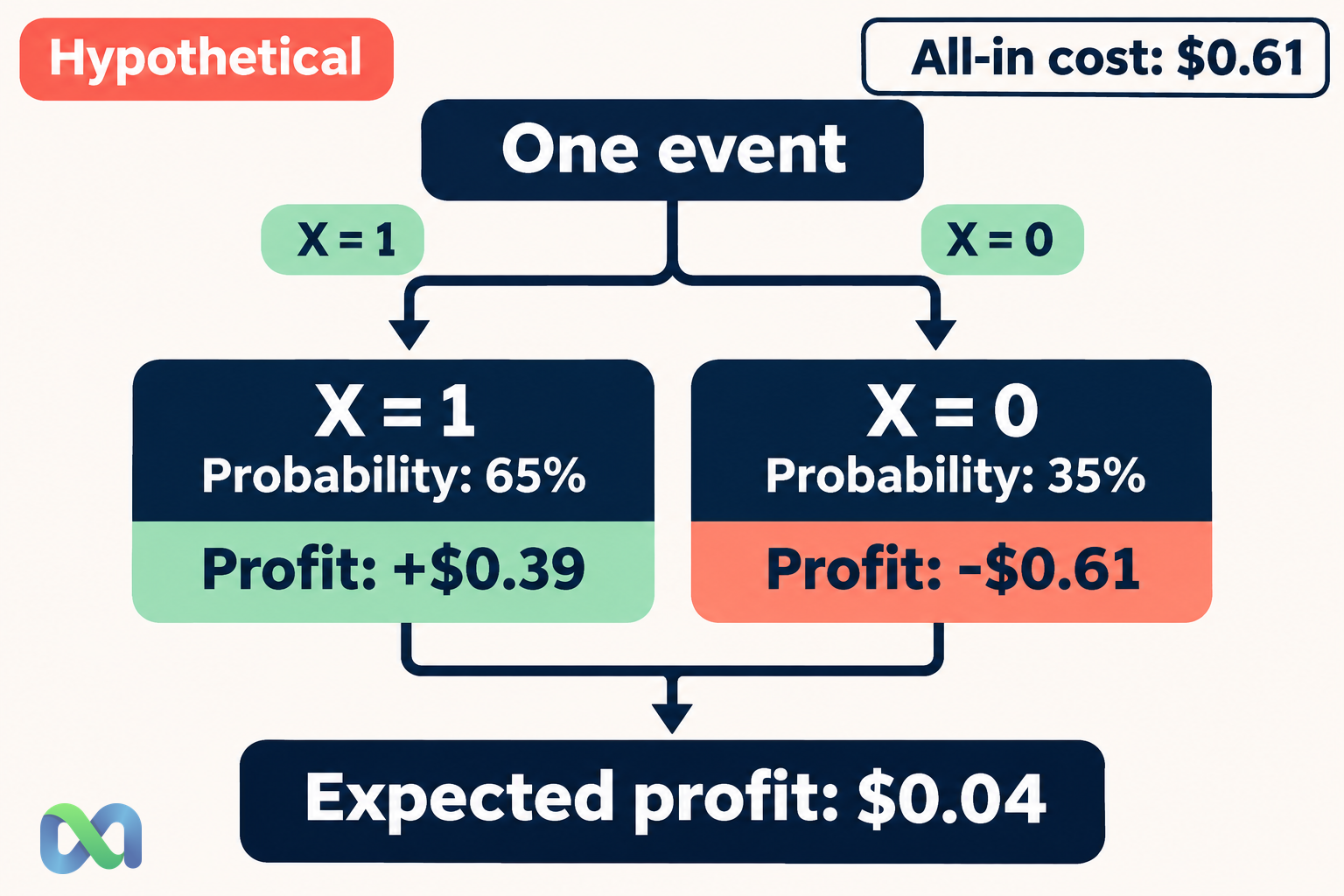
Suppose a hypothetical contract pays $1 when X = 1 and $0 when X = 0. Assume p = 0.65, an entry price of $0.60, and a fixed additional cost of $0.01.
These are generic teaching terms, not a representation of any particular Macro Markets contract. Verify actual payoff units, rules, fees, and settlement treatment separately.
Profit is the payoff minus the $0.61 all-in cost:
Profit = X − $0.61
| Outcome | Profit | Weight |
|---|---|---|
| Occurs | $0.39 | 65% |
| Does not occur | −$0.61 | 35% |
Expected profit is:
0.65 × $0.39 + 0.35 × (−$0.61) = $0.04
Equivalently, expected payout is $0.65, from which you subtract $0.61. Our expected value guide expands this probability-weighted approach.
Expected payout, profit, and return are different
The expected indicator is 0.65. The expected payout is $0.65. Expected profit is $0.04. Expected simple return on the assumed $0.61 all-in cost is about 6.56%.
Those numbers measure different things. The expected return also has no automatic annual meaning; the teaching example has not specified an investment horizon or a repeatable reinvestment process.
Subtracting the same fixed cost in both states does not change variance. Thus this dollar profit's variance is 0.2275 dollars squared. If the successful payoff were $10 rather than $1, the payoff variance would scale by 10².
State-dependent costs would require computing each state's net payoff directly. Do not assume they behave like the fixed cost used here.
Bernoulli vs Binomial Distribution
A Bernoulli variable describes one binary trial. A binomial variable counts successes across n independent Bernoulli trials with the same p.
The NIST binomial definition specifies those independent trials and common success probability. With n = 1, the binomial distribution reduces to Bernoulli.
If five independent events each have p = 0.65, their success count can take any whole-number value from zero through five. A single Bernoulli indicator cannot describe that whole count.
Contract units are not independent trials
Five units of the same contract settle according to one underlying event. Under the $1 teaching payoff, total proceeds are either $5 or $0, not every integer in between.
If total proceeds are 5X, their variance is 25p(1 − p). It is not 5p(1 − p), which would be the variance of a sum of five independent $1 payouts.
The independent events guide explains the distinction through joint probabilities. Real positions can lie between perfect dependence and independence, so their joint model needs evidence.
Estimating p and Checking Forecasts
For n observed binary trials with k successes, the sample success rate is k/n. For example, 13 successes in 20 trials gives 0.65.
That arithmetic does not prove the next event has a 65% chance. The estimate depends on whether the trials are comparable, how they were selected, and whether the probability process has changed.
A model that assigns different probabilities to different events also needs more than one pooled success rate. A group of 90% forecasts and a group of 40% forecasts should not be judged only by their combined average outcome.
Keep probability updates separate from payouts
New information can change p before the event settles. Our Bayes theorem guide explains one framework for updating a probability from evidence.
Changing a forecast is different from changing the event's payoff rule. For Macro Markets readers, keep the forecast, quoted entry value, resolution criteria, and net payoff calculation as distinct parts of the analysis.
This separation makes a simple Bernoulli model useful without pretending that it captures liquidity, execution, funding, or every exceptional settlement state.
Frequently Asked Questions
Can a Bernoulli variable have a value of 0.65?
No. Its realized value is zero or one. The parameter, mean, and an average across several observations can be 0.65.
Does Bernoulli require a 50/50 event?
No. Any p between zero and one is allowed. The symmetric 50/50 case is only one member of the family.
Are all binary financial contracts Bernoulli?
A clearly defined occurrence indicator can be Bernoulli. The financial payoff may be a transformation of it, or may require extra states for exceptional rules. Check the contract rather than assuming every feature is represented by one indicator.
Can two Bernoulli variables be dependent?
Yes. Each variable's marginal distribution can be Bernoulli while their outcomes depend on one another. A joint probability model is needed to describe that relationship.
