


Independent Events: Formula, Examples and When to Multiply Probabilities

Independent events are events where knowing that one happened does not change the chance of the other. Their joint probability follows the formula P(A ∩ B) = P(A) × P(B). The intersection symbol means “both events happen.”
The important part is the independence condition. Two market names, two different games or two separate headlines do not establish it. Before you multiply, check how your model links the two outcomes.
This guide explains the formula, compares independent and dependent events, and works through examples. All numerical forecasting scenarios are hypothetical teaching models. They are not current match forecasts, economic estimates, market quotes or evidence that a platform offers a particular trading product.
What Are Independent Events?
Two events are independent when news about one leaves the chance of the other unchanged. In a specified model of two independent fair coin tosses, knowing that the first toss was heads does not change the second toss's 50% chance of heads.
Independence is about what one event tells you about another. Events can happen at different times or in different places and still depend on each other. You can define independent events within one mathematical experiment, while events in different markets can depend on some of the same information.
The ProbabilityCourse chapter on independence gives the product definition and explains how it relates to conditional probability.
Independent versus dependent events
For independent events, knowing B leaves the chance of A unchanged, when that conditional chance is defined. For dependent events, knowing B changes it. The chance can rise or fall.
For example, drawing a red ball from a bag without replacing it changes the composition of the bag. The next draw faces a different set of possibilities. That is a clear reason to use a conditional probability.
In a real forecast, the link can be less clear. Write down the event definitions, relevant time periods and information already included in each estimate before treating the events as independent.
The Independent Events Probability Formula
For two independent events, use P(A ∩ B) = P(A) × P(B).
If A has probability 0.60 and B has probability 0.45, the joint probability under independence is 0.60 × 0.45 = 0.27, or 27%.
The result gives the chance that both events happen. The chance of at least one and the expected profit of a trade are separate questions.
Start from the general multiplication rule
When P(A) > 0, the general rule is P(A ∩ B) = P(A) × P(B | A).
Here, P(B | A) means the probability of B given that A occurred. Independence allows you to replace that conditional probability with the marginal probability P(B). Our conditional probability guide explains the notation and the change in the reference group.
You can also start in the other direction: P(A ∩ B) = P(B) × P(A | B), when P(B) > 0. Both versions describe the same overlap.
The product definition remains valid at probability zero or one. However, the elementary ratio used to define P(B | A) is undefined if P(A) = 0. In that case, the joint probability is zero because the intersection cannot be more probable than A.
“Both” and “at least one” are different questions
The general addition rule is P(A ∪ B) = P(A) + P(B) − P(A ∩ B). The union symbol means “A or B, including both.”
For the independent 60% and 45% example, the probability of at least one is 0.60 + 0.45 − 0.27 = 0.78, or 78%. Subtracting the overlap keeps you from counting the “both” cases twice.
Independent and Dependent Events: Worked Examples
The following examples use defined mathematical models or explicitly assumed forecasting probabilities. Keep the assumptions attached to each answer.
Two independent coin tosses
Assume two independent fair tosses. The four ordered outcomes are HH, HT, TH and TT. Each has probability one quarter. Let A mean heads on the first toss and B mean heads on the second.
Each event has probability 1/2. Their intersection is HH, so P(A ∩ B) = 1/4 = (1/2) × (1/2). The model's joint distribution establishes independence.
Two hypothetical games
Let A mean a specified team wins its game and B mean another team wins a different game. Assume P(A) = 60%, P(B) = 45% and independence for this exercise. The four outcome groups are:
| Outcome group | Probability |
|---|---|
| A and B | 27% |
| A only | 33% |
| B only | 18% |
| Neither | 22% |
For example, “A only” has probability 0.60 × 0.55 = 0.33. The four values total 100%. The “neither” category means neither specified win event occurs; depending on the sport, that can include a draw.
Different games do not prove independence. The table is correct under the stated model assumption, which needs support before applying it to actual matches.
Drawing without replacement
Take a hypothetical bag containing five red balls and five blue balls. Draw uniformly at random. If you replace the first ball and mix the bag before the next draw, the probability of red remains 5/10 on each draw.
Without replacement, a first red draw leaves four red balls out of nine. The chance of two reds becomes (5/10) × (4/9) = 2/9 ≈ 22.2%.
| Sampling method | Both red |
|---|---|
| With replacement | 25.0% |
| Without replacement | 22.2% |
Using 0.50 × 0.50 without replacement gives 25%, an overstatement of about 2.78 percentage points. You changed the answer by ignoring how the first draw affects the second.
When one event requires another
Imagine a tournament with a group stage followed by knockout rounds. Let A mean a team advances from its group and B mean it advances beyond the first knockout round. B cannot occur without A.
Assume P(A) = 0.70 and P(B | A) = 0.65. Then P(A ∩ B) = 0.70 × 0.65 = 0.455, or 45.5%. This is also P(B), since every B outcome includes A.
Multiplying the marginals instead gives 0.70 × 0.455 = 0.3185, or 31.85%. That answer is too low because it ignores the link: B needs A to happen first.
Independent Events Versus Mutually Exclusive Events
Independent events can occur together. The probability that both occur equals the product of their individual probabilities.
Mutually exclusive events cannot occur together: their intersection is empty. If both events have positive probabilities, they are dependent. Learning that one happened makes the other's probability zero.
Dependent events is the broader category where the independence equality fails. They may overlap, or they may be mutually exclusive.
For a simple example, suppose one fair die is rolled once. A is “the result is two” and B is “the result is five.” Each has probability 1/6, but the joint probability is zero. Multiplying 1/6 by 1/6 would incorrectly assign a positive probability to two different faces appearing on that single roll.
OpenStax distinguishes independence from mutual exclusivity and illustrates how replacement changes sampling.
There is an edge case: an event with probability zero can satisfy the independence product equality with another event. That is why the statement about mutually exclusive events being dependent needs the positive-probability condition.
How to Check Whether Events Are Independent
In a fully specified model, calculate P(A), P(B) and P(A ∩ B). Compare the joint probability with the product of the marginals. Equality establishes independence for that model.
When the relevant denominator is positive, you can instead compare P(B | A) with P(B), or P(A | B) with P(A). State which quantities you have and where they came from.
With real data, a sample gives you evidence about the wider population. An exact match in one sample does not prove independence in that population. The sample size, how you measured each event and changes over time can all affect the result.
Pairwise independence does not establish mutual independence
For three or more events, checking each pair does not justify multiplying all their individual chances. The product equality must hold for every relevant subset, including the full group.
Consider two independent fair coin tosses again. Define A as first toss heads, B as second toss heads and C as the two tosses matching. Each event has probability 1/2. Every pair has joint probability 1/4.
But all three happen together only for HH, with probability 1/4. Multiplying all three marginals gives 1/8. The events are pairwise independent, while the three-event set is not mutually independent.
What does zero correlation tell you?
For two event indicators with probabilities strictly between zero and one, zero population correlation is equivalent to independence of those two events. Their covariance equals P(A ∩ B) − P(A) × P(B), so setting it to zero gives the independence equality. This result is specific to the binary setting.
For other types of random variables, zero correlation need not mean independence. A zero estimate from a sample also does not prove independence in the wider population. State what you measured and how strong the evidence is.
Independent Events in Prediction Markets
Separate prediction markets can concern related outcomes. A hypothetical rate decision and a currency threshold, for example, may both be sensitive to economic news. A shared factor gives you a reason to check the link. It does not prove dependence on its own.
Compare two teaching models with the same marginals, P(A) = 60% and P(B) = 45%.
In the independent model, P(B | A) = 45%, so the joint probability is 60% × 45% = 27%.
In a dependent model, assume P(B | A) = 70% and P(B | not A) = 7.5%. These values keep B's overall chance at 45%: 0.60 × 0.70 + 0.40 × 0.075 = 0.45. But the joint probability is 60% × 70% = 42%.
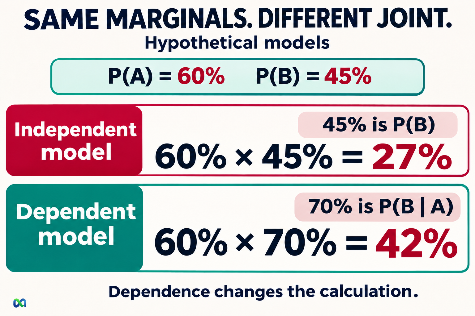
Knowing the chance of each event does not tell you the chance of both. In this example, both 27% and 42% are consistent with those marginals under different dependence assumptions.
Before you combine forecasts, read the outcome rules. Does one event require or rule out another? Does learning one change your estimate of the other? Write down your model assumption and the evidence for it.
The Bayes theorem guide explains how to update an estimate as new information arrives, including the need to retain information already observed. The expected value guide explains how a probability estimate enters a profit calculation.
A joint probability is a forecast input. It does not establish an executable price, available product or guaranteed return. Read the relevant market rules and evaluate the assumptions behind the numbers.
Frequently Asked Questions
When can you multiply probabilities directly?
You can multiply marginal probabilities to obtain the probability that both events occur when the events are independent in the model. Otherwise, use the general multiplication rule with an appropriate conditional probability.
Are independent events the same as unconnected events?
Independence is a mathematical relationship between probabilities. Different locations, dates or subject labels do not prove it. In a real forecasting problem, the absence of an obvious connection is not enough to establish independence.
Can independent events happen at the same time?
Yes. Independence means one event provides no information about the other's probability. It does not prohibit them from occurring together.
Does a losing streak make a win more likely?
In a model of independent trials with a fixed win probability, previous losses do not change the next trial's probability. Real market events may have changing probabilities or dependence, so you need to justify that model before applying it.
Can you assume independence when information is missing?
You can state it as a model assumption, but the answer then depends on that assumption. Missing evidence does not prove independence. Compare other ways the events might be linked to see how much your estimate could change.
