


Bayes Theorem: Formula, Examples and How to Update Probabilities

The Bayes theorem formula updates a probability when new evidence arrives. Its formula is P(H | E) = P(E | H) × P(H) / P(E), provided P(E) > 0. You combine an initial estimate with a model of the evidence to calculate a revised estimate.
For a forecaster, the useful question is: how much more likely is this information if my hypothesis is true than if it is false? A headline alone cannot supply that answer.
This guide explains the formula, works through two updates and shows why base rates matter. All numerical examples are hypothetical teaching models. The interest-rate scenario uses invented assumptions; it does not describe a real central-bank decision, economic release or market quote.
What Is Bayes’ Theorem?
Bayes’ theorem connects an initial probability, called the prior, to an updated probability, called the posterior. The update depends on how likely the observed evidence would be under the hypothesis and its alternatives.
The rule builds on conditional probability. P(H | E) means the probability of hypothesis H given evidence E. P(E | H) asks the reverse question: how likely would that evidence be if H were true?
The Bayes Theorem Formula
For evidence with positive probability:
P(H | E) = P(E | H) × P(H) / P(E)
The terms mean:
- P(H): your probability for H before incorporating E.
- P(E | H): the probability of observing E if H is true.
- P(E): the overall probability of observing E across the possible hypotheses.
- P(H | E): your probability for H after incorporating E.
For a binary hypothesis, let ¬H mean “H is false.” Then the denominator is P(E) = P(E | H) × P(H) + P(E | ¬H) × P(¬H).
This is the law of total probability: include the evidence that can arise in either group. The ProbabilityCourse chapter on Bayes’ rule gives the formula and its general form for a set of mutually exclusive, exhaustive hypotheses.
The formula organizes your assumptions. It does not tell you which starting probability or evidence model is justified.
Prior, Likelihood and Posterior Explained
The vocabulary becomes easier when you attach each term to a precise question.
Prior: what did you know before this evidence?
The prior describes your starting estimate for the defined event. It might draw on comparable past cases, an existing model or a documented judgment. Record the information it already includes.
A base rate can help if the historical cases are relevant. A rate-cut forecast, for example, needs more than a count of all past meetings. The policy setting, event definition and available information can affect whether those meetings are comparable.
You can examine a market price as an input to your thinking. But a price alone does not provide a complete evidence model. Our implied probability guide explains how to interpret prices and odds under stated assumptions.
Likelihood: how probable is the evidence under each case?
For a simple hypothesis, the likelihood term P(E | H) asks how often your specified signal would appear if H were true. Compare it with P(E | ¬H), the chance of that signal when H is false.
If both values are equal and positive, the signal does not change the probability of H. If the first is larger, the signal supports H within the model. If the second is larger, the signal supports ¬H.
Define the signal before estimating these values. “Weak jobs data” could mean payroll growth below a chosen threshold, a forecast miss or a rise in unemployment. Those are different conditions. Neither an adjective in a headline nor a market price gives you their likelihoods automatically.
Posterior: what changed after the evidence?
The posterior is the revised probability produced by your inputs. It remains a model estimate. Correct arithmetic does not establish that the inputs accurately describe the event.
For another update about the same hypothesis, this posterior can become your next prior. Carry forward the information already used as well as the number.
Bayes’ Theorem Example: Calculate an Updated Forecast
Consider a hypothetical central-bank decision. Define H as “the bank cuts its policy rate at a specified meeting.” Its complement, ¬H, includes decisions without a cut.
Let E1 be a jobs report meeting a predefined weak-data condition. For this exercise, assume:
| Assumption | Value |
|---|---|
| Initial chance of a cut | 40% |
| Weak data if a cut occurs | 65% |
| Weak data if no cut occurs | 35% |
These are teaching assumptions, not measured frequencies or a forecast for any real bank.
Step 1: identify the prior and its complement
The prior is P(H) = 0.40. Therefore P(¬H) = 1 − 0.40 = 0.60. Together, these two cases cover every outcome in the binary model.
Step 2: calculate the total probability of the evidence
The weak signal can appear whether or not a cut occurs. Include both routes:
P(E1) = 0.65 × 0.40 + 0.35 × 0.60
The first term is 0.26 and the second is 0.21. Their sum is 0.47.
Using only the first term in the denominator would leave out the weak-signal cases where there is no cut. That would answer the calculation incorrectly.
Step 3: divide the overlap by the evidence probability
P(H | E1) = 0.26 / 0.47 = 26/47 ≈ 55.3%
The estimate rises from 40% to about 55.3%. Under the stated assumptions, weak data is more likely when a cut occurs than when it does not.
You can check this with 1,000 equally weighted toy scenarios. There are 400 cut scenarios, of which 260 contain the weak signal. There are 600 no-cut scenarios, of which 210 contain it. Of the 470 signal scenarios, 260 involve a cut: 260/470 gives the same result.
Step 4: retain the exact result
Keep 26/47 for the next calculation. Use 55.3% to display the result. Rounding at every step can introduce an avoidable error into later updates.
Bayesian Updating With More Than One Signal
Now a second signal arrives: a hypothetical statement that meets a predefined hawkish-tone condition. In this exercise, hawkish means expressing greater concern about inflation. Call the signal E2.
You already know E1 occurred. The required likelihoods must reflect that history. Assume:
- P(E2 | H, E1) = 0.25: the chance of the statement given a cut and the weak-data signal.
- P(E2 | ¬H, E1) = 0.70: its chance given no cut and the weak-data signal.
The exercise specifies these conditional likelihoods directly. Bayes’ theorem does not require you to assume that the two signals are independent.
Use the probability of the second signal given the first
The prior for this stage is 26/47 for a cut and 21/47 for no cut. The denominator becomes:
P(E2 | E1) = 0.25 × (26/47) + 0.70 × (21/47)
This equals 21.2/47. The updated cut probability is:
P(H | E1, E2) = (0.25 × 26/47) / (21.2/47)
Canceling the common denominator gives 6.5 / 21.2 = 65/212 ≈ 30.7%.
| Stage | Cut estimate |
|---|---|
| Initial estimate | 40.0% |
| After weak jobs data | 55.3% |
| After hawkish statement | 30.7% |
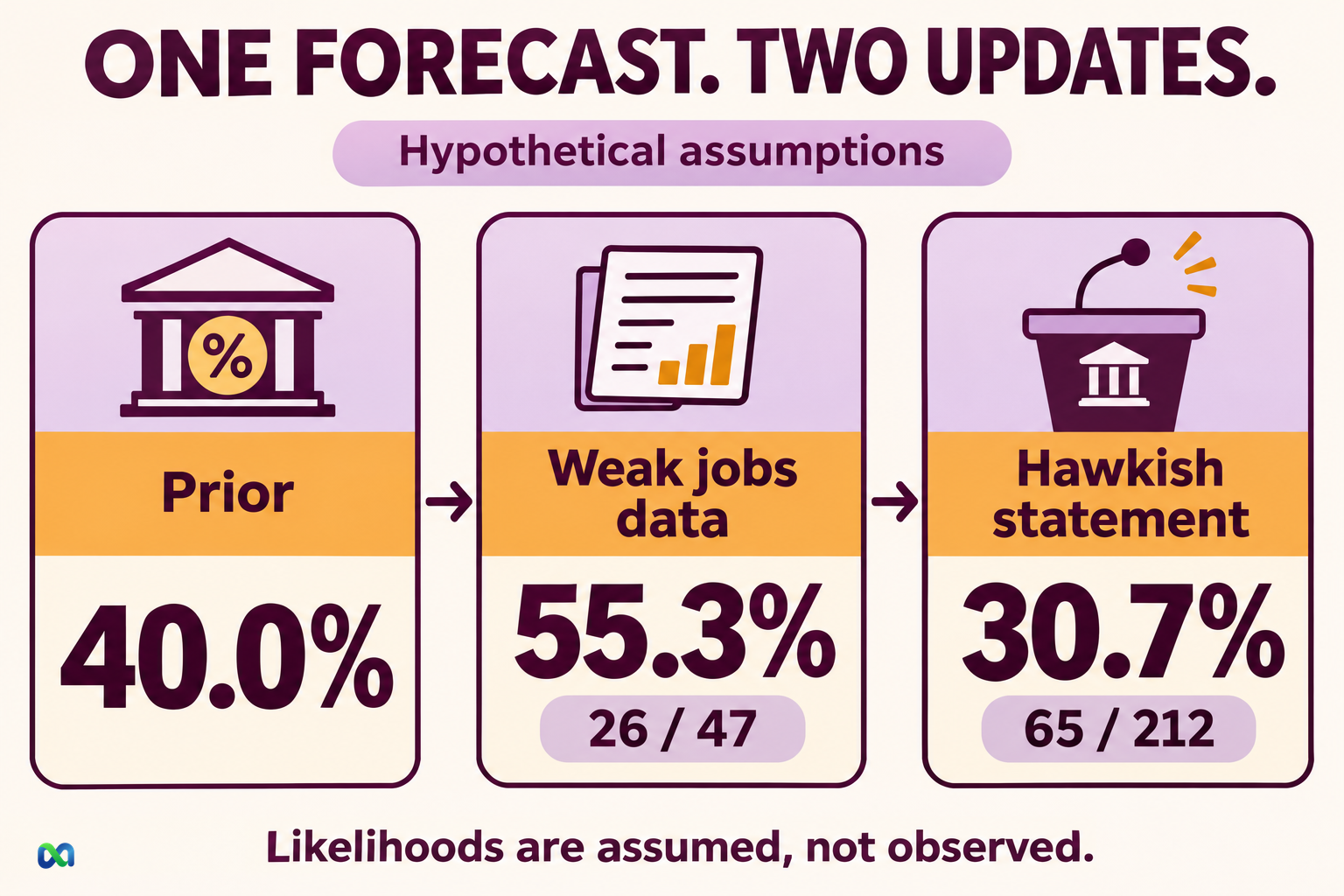
The second signal takes the estimate below the original 40%. That result follows from the assumed likelihoods; it is not a claim about how central banks respond to statements or jobs reports in practice.
Avoid counting the same information twice
A second article about the same report may add no evidence. If E2 is an exact copy of E1, observing it after E1 leaves the probability unchanged. For hypotheses still possible after E1, both conditional likelihoods of that copy are one.
For genuinely new information, estimate how likely it is under each hypothesis given what you already know. Replacing those values with unconditional likelihoods needs justification. The general update handles dependence by keeping the relevant history in the conditions.
Why Base Rates Matter in Bayes’ Theorem
A signal can strongly favor a hypothesis while leaving substantial uncertainty. To see why, take a separate toy example with a 5% prior for H.
Assume P(E | H) = 0.80 and P(E | ¬H) = 0.04. The evidence is 20 times as likely under H: the likelihood ratio is 0.80 / 0.04 = 20.
The denominator is 0.80 × 0.05 + 0.04 × 0.95 = 0.078. Bayes’ theorem then gives 0.04 / 0.078 = 20/39 ≈ 51.3%.
That is a large increase from 5%, but the result remains far from certainty. In 1,000 equally weighted toy scenarios, 50 satisfy H and 950 do not. The signal appears in 40 of the first group and 38 of the second. There are almost as many matching signals outside H as inside it.
The odds form provides another check
Probability p corresponds to odds p / (1 − p). For this binary example, the odds form of Bayes’ rule states:
Posterior odds = prior odds × likelihood ratio
Prior odds are 5/95 = 1/19. Multiplying by 20 gives posterior odds of 20/19. Converting back to probability gives (20/19) / (1 + 20/19) = 20/39.
Here, “odds” describes the ratio between the probabilities of H and ¬H in the model. Check the format before comparing that ratio with any quoted trading odds.
Base-rate neglect means leaving out relevant starting frequencies. A high P(E | H) alone cannot establish a high P(H | E). You also need the alternative likelihood and the prior.
Using Bayes in Prediction Markets
Begin with the exact event and resolution rule. A prediction market may specify a source, a deadline or a threshold. Build your hypothesis around that event so the probability answers the contract's question.
Next, separate the information already in your prior from the new signal. If you start from a price observed after a report, treating that report as a fresh update may count its information again.
Document where the likelihoods came from. Historical data, a model and a subjective assumption have different limits. If you cannot justify numerical inputs, Bayes’ theorem does not supply them for you. You can describe how evidence might matter without presenting an unsupported posterior as a measured chance.
Connect the estimate to a decision carefully
Your posterior is one input to a trading decision. An available execution price, contract payout, costs and risk constraints also matter. The expected value formula guide shows how a probability estimate enters a net-profit calculation.
A positive estimated expected value can disappear if the probability estimate is wrong or costs differ from your assumptions. Bayes’ theorem does not establish a platform's pricing method, guarantee liquidity or guarantee a profitable trade.
Keep a forecast journal with the event definition, timestamp, evidence source, prior, likelihoods and posterior. Preserve earlier entries instead of rewriting them after the outcome is known.
As events resolve, evaluate a series of forecasts. One correct call does not establish that the probabilities were well estimated. The Brier score guide explains how to measure probability-forecast error across resolved events.
Frequently Asked Questions
Is Bayes’ theorem the same as conditional probability?
Bayes’ theorem is an identity derived from conditional probability. It lets you calculate one conditional direction from the reverse direction and the relevant marginal probabilities. The terms P(H | E) and P(E | H) answer different questions.
Does Bayes’ theorem require independent evidence?
No. For successive updates, use the probability of each new signal conditional on the hypothesis and the evidence already observed. Conditional independence can simplify a model, but it is an extra assumption that needs support.
What happens if the evidence favors neither hypothesis?
If P(E | H) and P(E | ¬H) are equal and positive, their likelihood ratio is one. Posterior odds equal prior odds, so the probability stays unchanged.
Can the posterior become the next prior?
Yes, for a further update about the same hypothesis. Retain the full evidence history and enough numerical precision. In the worked example, use 26/47 rather than the displayed 55.3% in the second calculation.
Can Bayes’ theorem prove that a forecast is correct?
No. It gives a coherent update within the specified model. The event can still resolve against the higher-probability outcome, and the model itself may be poorly supported. Track assumptions and assess results over multiple forecasts.
