


Conditional Probability: Formula, Examples and Common Mistakes

Conditional probability is the probability of an event given that another event has occurred. The formula is P(A | B) = P(A ∩ B) / P(B), where P(B) must be greater than zero. Read it as “the probability of A given B.”
The key is the group you use as the base. Once you know B happened, you count only outcomes inside B. That change explains why a forecast can move after new evidence, and why reversing a question can produce a very different answer.
This guide works through the formula, a simple table, a prediction-market example and practice problems. Every numerical scenario below is hypothetical. The election counts illustrate the arithmetic; they are not polling data or a forecast for a real candidate.
What Does Conditional Probability Mean?
Suppose you roll a fair six-sided die. Before you see any information, three of the six faces are even. The chance of an even number is therefore 3/6, or 50%.
Now someone tells you that the result is greater than three. Only 4, 5 and 6 remain possible. Two of those three numbers are even, so the conditional probability is 2/3, or about 66.7%.
The die has not changed. The information has changed the set of outcomes you should consider. That is the main idea behind conditioning.
The conditional probability formula
Write the rule as P(A | B) = P(A ∩ B) / P(B).
- A is the event whose probability you want.
- B is the event you are conditioning on.
- P(A ∩ B) is the probability that both events happen. The intersection symbol means “and.”
- P(B) is the probability of the condition. It supplies the denominator.
For equally likely outcomes in a finite model, you can count cases instead: divide the number satisfying both A and B by the number satisfying B. If outcomes have different weights, use their probabilities rather than raw counts.
The conditional probability chapter in ProbabilityCourse gives this definition and its reduced-sample-space interpretation. The ratio requires P(B) > 0; dividing by zero does not give a valid answer.
How to Calculate Conditional Probability
Start by writing the question in words. What event do you want to estimate, and what information are you treating as known? Keep those roles fixed through the calculation.
Consider a toy model with 1,000 equally weighted election scenarios. Each scenario has two recorded features: whether the candidate wins and whether a particular poll signal is favorable. These counts are invented for this example.
| Poll signal | Wins / losses |
|---|---|
| Favorable | 450 / 150 |
| Not favorable | 50 / 350 |
| All scenarios | 500 / 500 |
Here, “not favorable” means the specified favorable signal is absent. It does not establish that there is an unfavorable poll. A neutral result, missing signal or other case could fall in that group, depending on the model's definition.
To find the probability of a win given a favorable signal:
- Define the target: A means the candidate wins.
- Define the condition: B means the favorable signal occurs.
- Count the cases in B: 450 wins plus 150 losses gives 600 scenarios.
- Count the overlap: 450 scenarios have both a win and the favorable signal.
- Divide: 450 / 600 = 0.75, or 75%.
You can get the same result with probabilities. The overlap is 450/1,000 = 0.45, and the condition has probability 600/1,000 = 0.60. Their ratio is 0.45 / 0.60 = 0.75.
Dividing 450 by all 1,000 scenarios would answer a different question. That result, 45%, is the joint probability of a win and a favorable signal.
The arithmetic is exact within this toy model. It does not establish that a real candidate has a 75% chance of winning. A useful real-world estimate needs a defensible model, relevant evidence and a clear definition of the outcome.
Conditional, Joint and Independent Events
These terms describe different questions. Keep the question attached to the number so you do not substitute one probability for another.
Marginal probability looks at one event without conditioning on the other. In the toy model, P(win) = 500 / 1,000 = 50%.
Joint probability asks whether both events happen. Here, P(win ∩ favorable signal) = 450 / 1,000 = 45%.
Conditional probability restricts the base to the stated condition. Here, P(win | favorable signal) = 450 / 600 = 75%.
The multiplication rule connects the last two: P(A ∩ B) = P(B) × P(A | B). In our example, 0.60 × 0.75 = 0.45. OpenStax explains the multiplication rule and its independence case.
What changes when events are independent?
If A and B are independent, learning that B occurred does not change the probability of A. When P(B) > 0, that means P(A | B) = P(A). Equivalently, P(A ∩ B) = P(A) × P(B).
The poll signal and win are dependent in our example: the conditional win probability is 75%, while the overall win probability is 50%. Their joint probability, 45%, also differs from 50% × 60% = 30%.
Do not confuse independence with mutual exclusivity. Mutually exclusive events cannot happen together. If two such events each have a positive probability, knowing one occurred makes the other's conditional probability zero.
Dependence alone does not prove causation. A signal can be related to an outcome without causing it. Nor does one favorable observation prove that a relationship will remain stable outside the model or sample used to estimate it.
Why P(A | B) and P(B | A) Can Differ
Reverse the question: among scenarios where the candidate wins, how often does the favorable signal occur?
The overlap is still 450. But there are 500 winning scenarios, so P(favorable signal | win) = 450 / 500 = 90%. The original calculation used 600 favorable-signal scenarios and produced 75%.
The numerator stayed the same. The denominator changed.
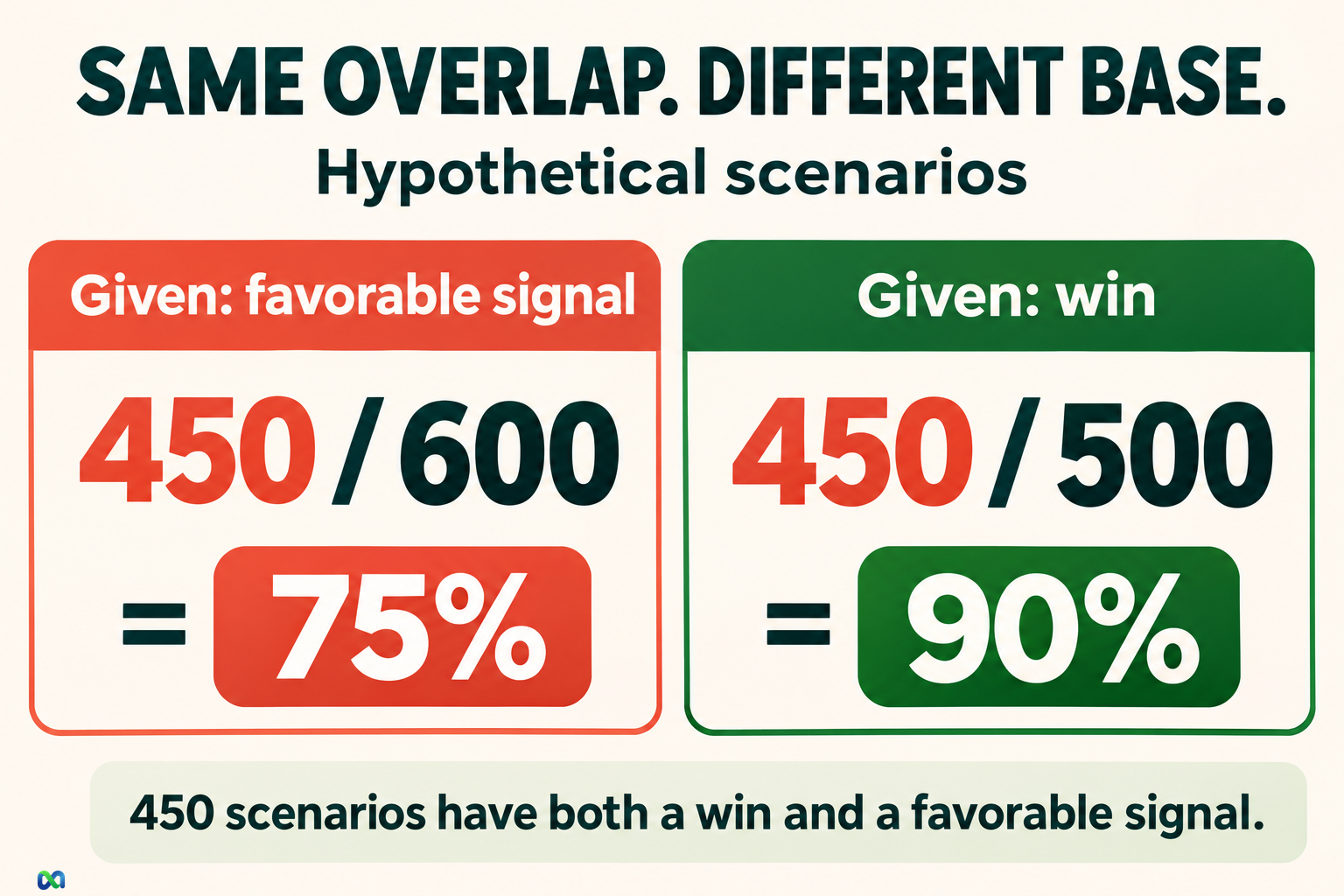
Use this check before dividing:
| Given information | Cases in the base |
|---|---|
| Favorable signal | 600 |
| Candidate wins | 500 |
| No favorable signal | 400 |
Treating P(B | A) as if it were P(A | B) is the inverse-probability error. A signal that appears often before a win may also appear often before a loss. To assess what the signal tells you, you need information about both groups.
The two conditional probabilities are not always different. They can coincide, including when the overlap is zero or when the two marginal probabilities are equal, provided both denominators are positive. The mistake is assuming equality without checking.
Where Bayes' theorem fits
Bayes' theorem connects the two directions using their base rates: P(A | B) = P(B | A) × P(A) / P(B), when P(B) > 0.
In the toy model, 0.90 × 0.50 / 0.60 = 0.75. Bayes' theorem gives the same answer as counting the 450 matching cases among the 600 favorable-signal cases. It does not turn an unreliable input into reliable evidence.
Ignoring a relevant base rate is a separate mistake from simply swapping the condition. Write down the original group sizes before using either shortcut.
Applying Conditional Probability to Prediction Markets
A prediction market concerns a specified outcome. Before updating a forecast, define A using the contract's actual resolution rule. Winning an election, being declared the winner by a named source and taking office can describe different events.
Then define B precisely. “Good news” is too vague to measure. “This poll's published margin is at least three points for the candidate” is a condition you could record and test. The same discipline applies to economic releases, sports results and other evidence.
Conditional reasoning helps separate three questions:
- What did I think before this information arrived?
- How does the information change my estimate for the specified event?
- How does that estimate compare with the price available to me?
A market price is not automatically your conditional probability. It is a trading input. Your model estimate is another input, and both can be uncertain. The implied probability guide explains how prices and odds translate into probability terms under stated assumptions.
For a hypothetical binary contract that pays $1 on a win and $0 otherwise, suppose the purchase price is $0.70. If your estimated win probability is 75%, expected gross payout is $0.75 per contract. With an assumed $0.01 total cost per contract, expected net profit would be $0.75 − $0.70 − $0.01 = $0.04.
Those inputs are invented, not a quote or fee schedule from Macro Markets or another platform. If your 75% estimate is poorly founded, the positive result says little about the opportunity. See the expected value formula guide for the distinction between expected profit and a realized result.
Keep a record of each update
Record the event definition, the information available at the time, the probability before and after the update, and your reason for changing it. Keep the first source of a claim separate from later articles that repeat it. Repeated coverage does not automatically provide independent evidence.
After outcomes resolve, evaluate a set of forecasts rather than judging your process from one trade. A correct result can follow a weak estimate, and a loss can follow a sensible estimate. The Brier score guide shows one way to measure probability-forecast error.
Conditional Probability Practice Problems
Try each question by writing the condition first. Then identify the cases or probability mass that belong in the denominator.
1. What if the favorable signal is absent?
Using the same hypothetical table, find P(win | no favorable signal).
Answer: There are 400 scenarios without the favorable signal, and 50 of them are wins. The result is 50 / 400 = 12.5%. It is not 50/1,000, because the question has already restricted the group.
2. Does independence make reversed conditionals equal?
Suppose P(A) = 0.60, P(B) = 0.25 and P(A ∩ B) = 0.15. Find both conditional probabilities and check independence.
Answer: P(A | B) = 0.15 / 0.25 = 0.60. In the other direction, P(B | A) = 0.15 / 0.60 = 0.25. Since 0.60 × 0.25 = 0.15, the events are independent. Each conditional equals its own marginal probability; the reversed conditionals still differ.
3. Can new information leave a probability unchanged?
Suppose P(A) = 0.50. A signal E has a 60% chance of appearing when A occurs and a 60% chance when A does not occur. What is P(A | E)?
Answer: P(E) = 0.60 × 0.50 + 0.60 × 0.50 = 0.60. The overlap P(A ∩ E) is 0.50 × 0.60 = 0.30. Therefore P(A | E) = 0.30 / 0.60 = 50%. In this model, the signal does not distinguish A from its opposite.
Frequently Asked Questions
What does the vertical bar in P(A | B) mean?
It means “given.” P(A | B) asks for the probability of A within the outcomes where B has occurred. The event after the bar determines the reference group.
Is conditional probability the same as joint probability?
No. Joint probability asks how likely A and B are together across the whole sample space. Conditional probability asks how likely A is after restricting attention to B.
Can conditional probability be greater than the original probability?
Yes. In the die example, P(even) is 50%, while P(even | greater than three) is about 66.7%. Depending on the condition, the probability can rise, fall or stay the same. A valid conditional probability still lies between zero and one.
What if the probability of the condition is zero?
The elementary ratio P(A ∩ B) / P(B) is undefined when P(B) = 0. Do not enter zero in the denominator and report a percentage. More advanced probability models handle some zero-probability conditioning questions using other methods.
Does a favorable signal guarantee a favorable outcome?
No. Even the toy model's 75% conditional probability leaves a 25% probability of losing within that group. A forecast expresses uncertainty about an event; it does not promise the event or a profitable trade.
