


Binomial Distribution: Formula and Examples

A binomial distribution gives the probability of getting a specified number of successes in a fixed number of independent trials. Each trial has two outcomes, and its success probability stays the same throughout the model.
For example, suppose five independent events each have a hypothetical 60% chance of occurring. The binomial distribution can calculate the chance that exactly three occur. It cannot establish whether 60% is a good forecast or whether those events really are independent.
This guide explains the formula, works through the full probability table, and connects the result to binary contracts. All probabilities and contract amounts below are teaching assumptions, not live prices or observed trading results.
What Is a Binomial Distribution?
The binomial distribution models a count of successes across n trials. A success is simply the outcome being counted. It does not have to mean a profitable trade, a good result, or a correct forecast.
Write X ~ Binomial(n, p). Here, X is the success count, n is the fixed number of trials, and p is the probability of success on each trial. Possible values of X are the whole numbers from zero through n.
The NIST definition of a binomial distribution specifies independent Bernoulli experiments with a common success probability. One Bernoulli trial produces a zero or a one; the binomial variable adds those outcomes.
If you count how many of five events occur, the answer could be zero, one, two, three, four, or five. It cannot be 2.7. A model's average count can be fractional even though every individual count is a whole number.
Check the four conditions first
Use a fixed number of trials, two clearly defined outcomes per trial, independent trials, and the same success probability for each trial. Define what counts as success before observing the results.
Independence is a substantive assumption. Five positions linked to the same announcement may move or settle together. Our guide to independent events explains why separate labels do not establish independence.
Stopping after the third success also changes the question. That is a random number of trials, rather than the fixed-five-trial experiment used here.
The Binomial Distribution Formula
The probability of exactly k successes is:
P(X = k) = C(n, k) × p^k × (1 − p)^(n − k)
The combination term is:
C(n, k) = n! ÷ [k! × (n − k)!]
A factorial multiplies the positive integers up to its argument. For example, 3! = 3 × 2 × 1 = 6. By convention, 0! = 1. The NIST distribution reference gives this probability formula and its cumulative counterpart.
The term p^k × (1 − p)^(n − k) gives the probability of one particular ordering of successes and failures. C(n, k) counts how many orderings have the same success count.
For three successes in five trials, there are 10 possible orderings. Counting only success-success-success-failure-failure would omit the other nine. Under the independence and common-probability assumptions, all 10 have the same probability.
The formula also handles the endpoints. Exactly zero successes has probability (1 − p)^n. Exactly n successes has probability p^n. When p is zero or one, the count is certain and has no variation.
A Worked Example: Five Trials at 60%
Assume n = 5 and p = 0.60. To find the probability of exactly three successes, first calculate the combinations:
C(5, 3) = 5! ÷ (3! × 2!) = 10
Then substitute the probabilities:
P(X = 3) = 10 × 0.60³ × 0.40² = 0.3456
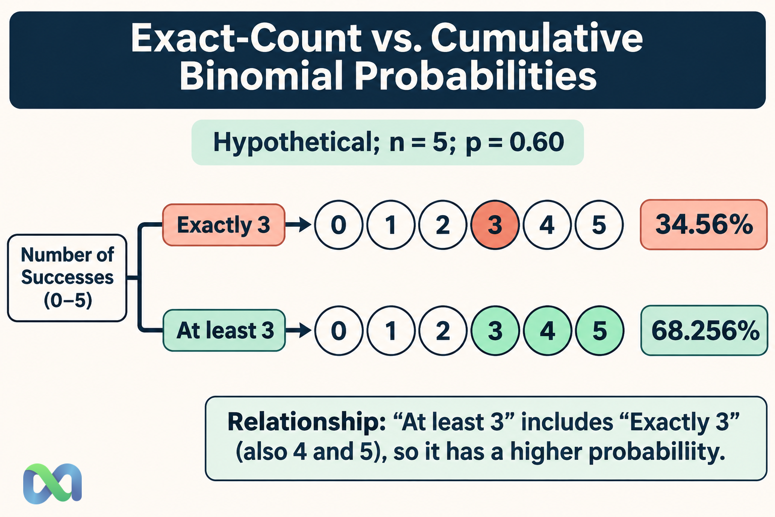
The result is 34.56%. This is the probability of exactly three successes, not three or more.
The complete probability table
Applying the same calculation to each possible count gives:
| Successes | Probability |
|---|---|
| 0 | 1.024% |
| 1 | 7.680% |
| 2 | 23.040% |
| 3 | 34.560% |
| 4 | 25.920% |
| 5 | 7.776% |
The six probabilities sum to 100%. Three successes is the most likely count in this example, but its probability is still below 50%. The most likely individual outcome need not account for most of the total probability.
Exactly, at least, and at most
For at least three successes, add the probabilities of three, four, and five:
P(X ≥ 3) = 34.560% + 25.920% + 7.776% = 68.256%
For at most two, add zero, one, and two:
P(X ≤ 2) = 1.024% + 7.680% + 23.040% = 31.744%
These are complementary events, so their probabilities add to 100%. “At least three” includes three; “more than three” includes only four and five, giving 33.696%. Small wording changes can change the answer substantially.
Mean, Variance, and Standard Deviation
For a binomial count, the mean is np, the variance is np(1 − p), and the standard deviation is the square root of that variance.
In the five-trial example:
Mean = 5 × 0.60 = 3 successes
Variance = 5 × 0.60 × 0.40 = 1.20 successes²
Standard deviation = √1.20 ≈ 1.095 successes
The mean describes an average across repetitions of the whole five-trial experiment. It does not promise three successes in the next batch. The table assigns a combined 65.44% probability to counts other than three.
The standard deviation summarizes spread around the mean. It is not an error bound and does not make the count normally distributed. With only five trials, the exact discrete probabilities are straightforward to calculate and avoid approximation issues.
At a fixed n, variance is largest when p = 0.50. A probability near zero or one makes the count more concentrated, but whether that probability is realistic remains a separate modeling question.
Using the Model for Binary Contracts
Consider a hypothetical portfolio with one contract on each of five independent events. Each contract pays $1 if its event occurs and $0 otherwise. Assume every event has probability 0.60, each contract costs $0.55, and all positions are held to settlement.
These are generic teaching terms, not a description of a specific Macro Markets contract. Actual settlement rules, currencies, fees, and access conditions must be checked separately.
The total entry cost is $2.75. With X successful events, total settlement proceeds are X dollars:
Profit before costs = X − $2.75
Profit is positive when X is at least three. Under the stated model, that probability is 68.256%. Expected proceeds are $3, so expected profit before costs is $0.25.
A fixed total cost of $0.05 would reduce expected profit to $0.20 and change the profit expression to X − $2.80. It would not change this example's minimum profitable count of three. Other costs or entry prices could change that threshold.
Our expected value guide explains the distinction between average profit and the chance of profit. Neither number guarantees the next result.
Five contracts can still be only one trial
Buying five contracts on the same binary event does not create five independent trials. Under the teaching payoff above, all five pay together or all five pay zero. The total payout is then either $5 or $0.
Treating that exposure as Binomial(5, 0.60) would invent intermediate settlement outcomes that cannot occur. Position quantity and the number of independent events are different inputs.
Even contracts on different events can depend on a shared economic driver. Before applying the binomial formula, ask what could make several positions settle the same way.
Spreadsheet Calculation and Model Checks
Using Excel’s BINOM.DIST function, the exact-three calculation is:
=BINOM.DIST(3,5,0.6, FALSE)
The cumulative probability through two successes is:
=BINOM.DIST(2,5,0.6, TRUE)
For at least three, subtract that cumulative probability from one:
=1-BINOM.DIST(2,5,0.6, TRUE)
These formulas return decimal probabilities: 0.3456 and 0.68256, respectively. Format the cells as percentages if desired. Some spreadsheet locales use a different argument separator.
Before interpreting the answer, check that n is a nonnegative whole number, k lies between zero and n, and p lies between zero and one. Sum the full probability table when feasible. A total far from one suggests an input, formula, or rounding problem.
What to do when the assumptions fail
Different probabilities across independent trials require a model such as the Poisson binomial distribution. Sampling without replacement from a small fixed population can call for a hypergeometric model. Dependent events require a joint model that preserves that dependence.
Use conditional probability to express how one event or new piece of information changes another event’s probability. That is a different question from counting successes under a fixed independent-trial model.
These alternatives answer different questions. Do not average several probabilities and assume the resulting binomial model preserves their full count distribution.
For prediction market analysis, record the event definitions, common-probability assumption, source of the forecast, and reason for treating events as independent. A precise calculation is useful only when it represents the exposure being assessed.
Frequently Asked Questions
What is the difference between Bernoulli and binomial?
A Bernoulli variable records one binary trial as zero or one. A binomial variable counts successes across a fixed number of independent Bernoulli trials sharing the same probability. The binomial distribution with n = 1 is Bernoulli.
Does a 60% probability mean exactly 60% of trials succeed?
No. It is the assumed chance on each trial. The realized success share varies, especially in small samples. The five-trial table illustrates that variation directly.
Is a binomial distribution always symmetric?
No. With 0 < p < 1, it is symmetric when p = 0.50 and generally skewed otherwise. The size of n also affects its shape. A bell-shaped sketch should not replace the exact probabilities for a small count.
Can a market price be used as p?
A displayed price can be a modeling input after considering the contract, costs, liquidity, and interpretation. It does not independently prove the event's true probability. Keep a quoted price separate from the forecast probability used in the calculation.
