


Conditional Value at Risk (CVaR): Formula and Examples
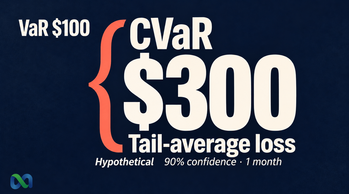
Conditional value at risk, or CVaR, measures the average loss in a chosen worst-case share of a loss distribution. At 90% confidence, it averages the worst 10% of outcomes under the stated model and time horizon.
It answers a different question from value at risk, or VaR. VaR identifies a loss threshold. CVaR describes the losses in the tail beyond that threshold, with care needed when several outcomes share the threshold value.
This guide explains the conditional value at risk formula and works through a hypothetical example. The probabilities and dollar amounts are teaching inputs, not market quotes, forecasts, or a claim about any platform's historical performance.
What Is Conditional Value at Risk?
CVaR summarizes the average loss across the worst specified share of outcomes. That share is often called the loss distribution's tail.
This guide uses a loss convention: positive numbers are losses, zero means no gain or loss, and negative numbers are gains. A loss of −$100 therefore means a $100 gain. Larger values represent worse financial outcomes.
Set the time horizon before calculating. A one-month dollar loss and a one-day percentage loss are different inputs. Neither the confidence level nor the CVaR number makes the underlying model correct.
CVaR and expected shortfall
Expected shortfall, or ES, is a common name for the tail-average measure used here. The CFA Institute discussion of extreme downside risk uses these related terms.
Naming alone does not settle the calculation. Some explanations define CVaR as a conditional average of losses strictly above VaR. That shortcut works in suitable continuous distributions, but can fail for discrete outcomes.
We use the general-distribution definition developed by Rockafellar and Uryasev. It fills exactly the required tail probability, including an appropriate part of the probability at VaR when needed. Their paper on general loss distributions explains why that distinction matters.
Our risk and analytics glossary provides related terms. The worked example below makes the probability weighting explicit.
CVaR vs VaR: What Is the Difference?
For confidence level α, VaR is the smallest loss amount whose cumulative probability is at least α. In plain terms, sort losses from best to worst and find where the required probability has been covered.
CVaR then averages the worst 1 − α share of probability. At 90% confidence, the tail is 10%. At 95%, it is 5%.
VaR is not the maximum loss that can happen. Losses above it remain possible. CVaR gives more information about their size, but it is also an average rather than a cap.
A confidence level is part of the model
At a chosen horizon, a 90% VaR of $100 means the model assigns at least 90% probability to losses no greater than $100. In a discrete model, the covered probability can exceed 90% because a whole group of outcomes shares the threshold.
A 90% CVaR of $300 means the worst 10% tail has an average loss of $300 under that model. It does not mean a 90% chance of losing $300, or a 90% chance that the estimate itself is accurate.
Specify the confidence level, horizon, units, positions, and source of the probabilities. Comparing unlabeled numbers can mix different questions.
The Conditional Value at Risk Formula
For a finite set of loss scenarios, the tail-weighted calculation is:
CVaR = sum(loss × probability included in the tail) ÷ tail probability
The included probabilities must add up to 1 − confidence level. Start with the largest loss, then work toward smaller losses until that tail is full.
Use all of a scenario's probability if it fits. If the next scenario would overfill the tail, use only the portion required. This splits probability for the calculation; it does not split a position or change the loss amount.
A formula that also handles discrete losses
Rockafellar and Uryasev's original optimization paper introduced a useful calculation, which their later general-distribution paper extends:
CVaR at confidence α = minimum over t of {t + E[max(loss − t, 0)] ÷ (1 − α)}
Here, t is a candidate loss threshold. The max operation keeps only positive amounts above it. E means the probability-weighted average over all scenarios. Find the lowest value of the full expression as t varies.
This formula provides a separate way to check the tail average. It does not mean choosing an arbitrary threshold and assuming the result is CVaR. For the example below, a minimizing threshold is the VaR value of $100.
How to Calculate CVaR: A Worked Example
Assume the following one-month portfolio loss model. Amounts are in U.S. dollars and already include the costs assumed in this hypothetical example. The four probabilities add up to 100%.
| Loss | Weight | Cumulative |
|---|---|---|
| −$100 | 40% | 40% |
| $0 | 40% | 80% |
| $100 | 15% | 95% |
| $500 | 5% | 100% |
The first row is a gain. The cumulative column counts probability from the smallest loss upward. These weights are assumed model probabilities, not measured frequencies or a live forecast.
Step 1: Find the 90% VaR
At a loss of $0, cumulative probability is 80%, below the required 90%. At $100, it reaches 95%. The smallest loss reaching at least 90% is therefore $100.
The 90% VaR is $100 even though this discrete threshold covers 95% of the model's probability. Do not interpolate between $0 and $100 without declaring a different quantile convention.
Step 2: Fill the worst 10% tail
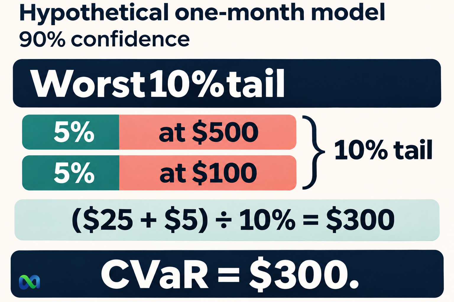
The $500 loss accounts for 5% probability. Include all of it. The tail still needs another 5 percentage points of probability to reach 10%.
The next loss is $100, with 15% probability available. Include only 5 percentage points from that group. That is one-third of its probability, not one-third of its dollar loss.
The required tail now contains 5% at a $500 loss and 5% at a $100 loss.
Step 3: Calculate the weighted average
Use probabilities as decimals:
90% CVaR = (0.05 × $500 + 0.05 × $100) ÷ 0.10
= ($25 + $5) ÷ 0.10 = $300
The $30 numerator is the tail's contribution to average loss across the whole distribution. Dividing by its 10% probability turns that into the average within the tail. Reporting $30 as CVaR would omit this normalization.
Check the result using the threshold formula
At t = $100, only the $500 scenario has a positive amount above the threshold. That amount is $400 and its probability is 5%:
E[max(loss − $100, 0)] = 0.05 × $400 = $20
$100 + $20 ÷ 0.10 = $300
Both methods give the same answer. CVaR averages total losses in the tail, rather than only the dollars above VaR.
Why averaging every loss at VaR is wrong here
All outcomes at or above $100 have 20% total probability. Averaging all of them gives $200. Taking only losses strictly above $100 gives $500.
Neither is the required 90% CVaR of $300. The requested tail is 10%, so it needs only part of the probability at $100. Counting scenarios equally would also be wrong because their assigned probabilities differ.
How to Interpret Expected Shortfall
Under the same model, horizon, and confidence level, a larger CVaR means a larger average loss in the selected tail. Dollar values also depend on position size, so match the exposure before comparing portfolios.
A smaller CVaR does not establish which portfolio will earn more. It does not describe every feature of the return distribution or replace an assessment of the model's inputs.
Changing confidence can change CVaR while VaR stays the same
At 95% confidence, the table still gives VaR of $100. The required worst 5% tail, however, consists entirely of the $500 scenario. Its average loss is $500.
| Measure | 90% | 95% |
|---|---|---|
| VaR | $100 | $100 |
| CVaR | $300 | $500 |
These are one-month dollar values for the same hypothetical portfolio. The unchanged VaR does not mean the two confidence levels ask the same question. CVaR highlights the different tail being averaged.
CVaR is not a worst-case limit
At 90%, this example's CVaR is $300 while its largest listed loss is $500. At 95%, CVaR happens to equal that model's largest loss. Neither result proves that the model includes every loss that could occur in reality.
A historical sample can omit rare events. A scenario model can leave out an important joint outcome or assign it too little probability. More decimal places do not fix those gaps.
Limits for Prediction Market Portfolios
Binary settlement and a limited set of portfolio outcomes can create discrete losses. That makes probability at the VaR boundary relevant. A smooth curve drawn over those outcomes does not remove the need to choose a suitable calculation.
A single contract price is not a complete portfolio loss model. Define the positions, entry costs, settlement outcomes, and time horizon first. Keep forecast probabilities separate from assumptions about execution and account values.
Joint outcomes and executable losses
Positions tied to the same event can lose together. Adding each position's separate CVaR does not, in general, calculate portfolio CVaR. Build a joint loss model that accounts for how the outcomes relate.
Fees, spreads, liquidity, and position size may affect the proceeds available on exit. State whether scenarios use settlement payoffs, displayed marks, or estimated executable prices. Apply the same cost treatment throughout.
Changing from one month to a year also requires a suitable loss model for the new horizon. Do not treat twelve times a monthly CVaR as a universal annual conversion.
Keep return and drawdown measures alongside it
The Sortino ratio compares average return above a target with downside deviation. The Sharpe ratio compares excess return with its variation. Neither is a dollar tail-loss estimate.
Maximum drawdown measures a fall from an earlier peak along a portfolio value path. CVaR for a chosen horizon does not directly describe that path or recovery time.
For Macro Markets readers, these distinctions help separate market forecasts, portfolio losses, and historical performance. CVaR is one view of risk, not a rule that decides whether a position should be opened or increased.
Frequently Asked Questions
Is CVaR the same as expected shortfall?
They commonly name the same tail-average measure. Check the definition when using software or comparing reports. For discrete losses, an average of outcomes strictly above VaR can differ from the general-distribution CVaR used here.
Is CVaR always greater than VaR?
With the same loss convention, model, horizon, and confidence level, this CVaR is at least as large as VaR. Equality can occur. That relationship does not make either number a guaranteed loss bound.
Does a 95% CVaR mean a 95% chance of losing that amount?
No. It is the average loss in the worst 5% tail under the chosen model. It does not state that the average amount itself has 95% probability of occurring.
How much historical data is enough?
There is no universal sample size that guarantees a reliable tail estimate. Short samples contain little information about rare losses. Consider the frequency, horizon, market conditions, missing observations, and whether the sample represents the risks being modeled.
