


Confidence Interval: Formula, Examples and Interpretation
A confidence interval describes uncertainty around an estimated population parameter. It combines a sample estimate, a measure of sampling variability, and a confidence level chosen for the calculation. Its meaning depends on how the data were collected and on whether the statistical model is appropriate.
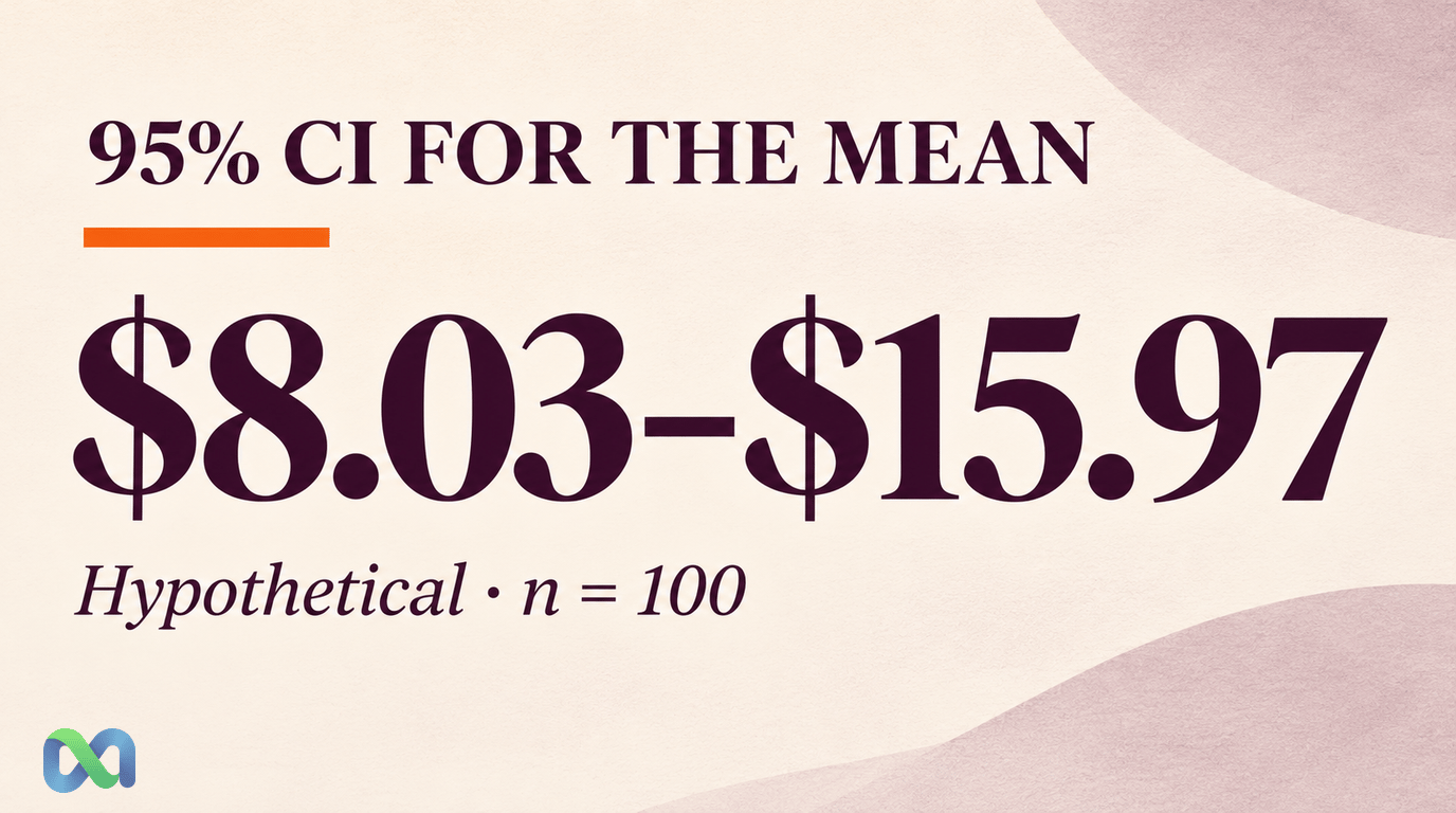
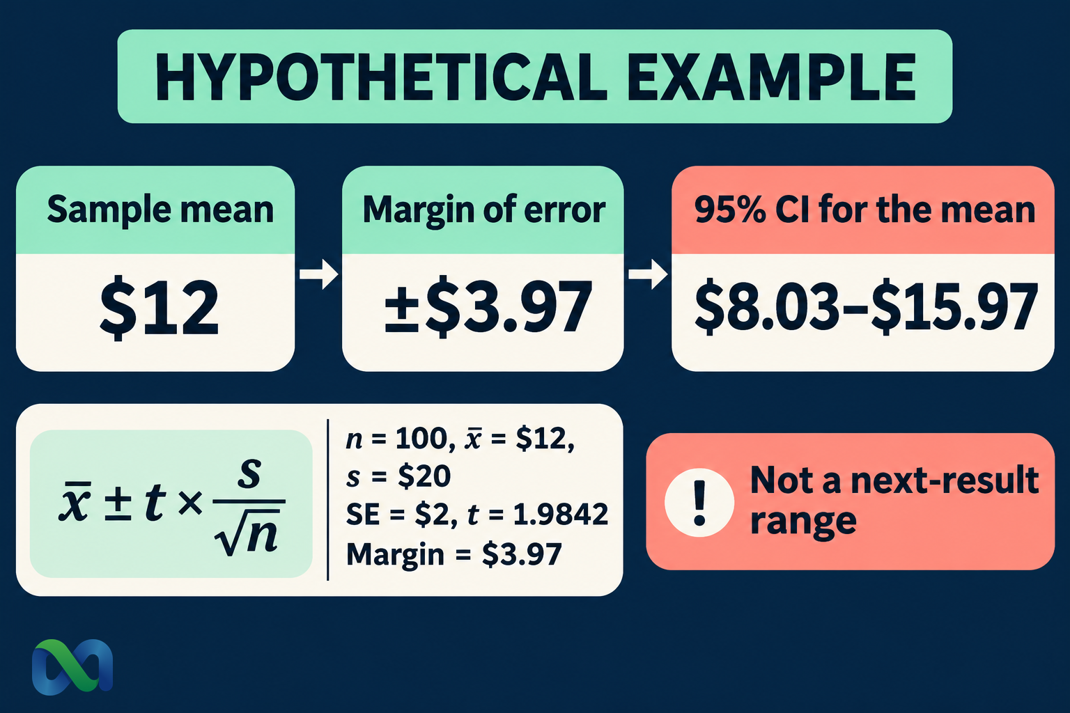
Suppose a hypothetical sample of 100 independent positions has an average net result of $12 and a sample standard deviation of $20. A conventional 95% t-interval for the population mean is approximately $8.03 to $15.97, under the assumptions explained below. That interval concerns an average. It does not describe where the next position will finish.
This guide shows how to calculate and interpret a confidence interval, how sample size affects its width, and how to distinguish it from a prediction interval. All results are teaching examples rather than Macro Markets trading data.
What Is a Confidence Interval?
A confidence interval supplies a lower and an upper limit for an unknown population quantity. The quantity could be an average transaction cost, a mean forecast error, or a proportion of events that resolve a particular way. The formula must match the quantity being estimated.
The confidence level belongs to the procedure. If a valid 95% procedure were applied repeatedly to new samples collected in the same way, approximately 95% of the resulting intervals would contain the fixed population parameter. A particular interval either contains that parameter or does not. NIST explains this repeated-sampling interpretation.
It is therefore misleading to say that 95% of individual results fall inside a confidence interval for the mean. Those individual results can be much more dispersed than their average. It is also misleading to treat the confidence level as the probability that a trading strategy will succeed.
A narrow interval indicates precision under the model. It does not establish that the sample represents the population you care about. A precise estimate from a biased sample can still be systematically wrong.
The Confidence Interval Formula for a Mean
When the population standard deviation is unknown, a common two-sided interval is:
Sample mean ± t critical value × sample standard deviation ÷ √n
In symbols, this is x̄ ± t × s/√n. Here, x̄ is the sample mean, s is the sample standard deviation, and n is the number of observations. The t critical value uses n − 1 degrees of freedom and the selected confidence level.
The expression s/√n is the estimated standard error of the mean. Multiplying it by the critical value produces the margin of error. Subtract that margin from the estimate to obtain the lower limit; add it to obtain the upper limit.
OpenStax’s t-interval reference distinguishes the t-interval from the z-interval used when the population standard deviation is known. Replacing an unknown population standard deviation with a sample estimate is a reason to use the t distribution.
For independent normal observations, this t-interval has its stated coverage. With nonnormal observations, its suitability depends on sample size, tail behavior, and dependence. “There are 100 rows” is not sufficient evidence that a financial dataset satisfies those conditions.
Worked Example: A 95% Confidence Interval
Assume the following hypothetical sample summary: n = 100, x̄ = $12, and s = $20. For the benchmark calculation, assume independent observations from a normal population with a stable mean and variance. This specifies a mathematical example; it is not a description of actual trading returns.
First, calculate the standard error:
SE = $20 ÷ √100 = $2
For a two-sided 95% interval with 99 degrees of freedom, the t critical value is approximately 1.9842. The margin of error is:
Margin = 1.9842 × $2 ≈ $3.97
The interval is therefore:
$12 ± $3.97 = approximately $8.03 to $15.97
Under this model, the data support an estimate of the population mean with that interval. They do not establish that an individual position will return between $8.03 and $15.97. They also say nothing about omitted fees unless those fees were included in every observation.
Change the confidence level
Keeping the sample summary fixed gives the following intervals. Calculations use the t distribution rather than rounding every critical value to a normal approximation.
| Level | Margin | Mean CI |
|---|---|---|
| 90% | $3.32 | $8.68 to $15.32 |
| 95% | $3.97 | $8.03 to $15.97 |
| 99% | $5.25 | $6.75 to $17.25 |
Higher confidence produces a wider interval from the same data. You are asking the procedure to cover the parameter more often, so it must allow more uncertainty. Choosing a lower confidence level after seeing an inconvenient result changes the reporting rule and should be disclosed.
What Makes the Interval Wider or Narrower?
Three direct inputs control the width: the confidence level, the sample standard deviation, and the sample size. More variable observations produce a wider interval. A larger independent sample generally produces a narrower one, assuming a comparable data-generating process.
The square-root relationship matters. With a stable population standard deviation, multiplying sample size by four roughly halves the standard error. Collecting twice as much data does not generally halve it. The t critical value also changes with the degrees of freedom.
Suppose a hypothetical analysis holds x̄ = $12 and s = $20 fixed while comparing possible sample sizes:
| n | SE | 95% CI |
|---|---|---|
| 25 | $4.00 | $3.74 to $20.26 |
| 100 | $2.00 | $8.03 to $15.97 |
| 400 | $1.00 | $10.03 to $13.97 |
These are sensitivity calculations, not a promise that future data will retain the same mean and dispersion. Adding observations can reveal a regime change, a data-quality problem, or previously unseen losses. Read the standard deviation guide for the distinction between the spread of observations and uncertainty about their mean.
Confidence Interval vs. Prediction Interval
A confidence interval for the mean estimates the population average. A prediction interval addresses a future observation under a specified model. A credible interval has a Bayesian interpretation conditional on its model, prior, and observed data. These intervals answer different questions.
In the worked example, the estimated standard error is $2 while the sample standard deviation is $20. Averaging 100 independent observations reduces sampling variation in the mean. It does not remove the variation in the next result. A prediction interval for one new observation would usually be substantially wider than the confidence interval for the mean.
Similarly, a confidence interval for an event frequency is not automatically a probability range for the next named event. Events with different underlying probabilities are not interchangeable Bernoulli trials. Their subject matter, information set, and settlement rules can differ.
When evaluating a prediction-market position, start with the actual contract, forecast, price, and costs. Our expected value explanation covers the payoff calculation. Confidence intervals can describe uncertainty in an estimated input, but they do not supply a market price or turn historical averages into a guaranteed edge.
Calculate the Interval in a Spreadsheet
Suppose the 100 hypothetical net results occupy cells A2:A101. Calculate the mean with =AVERAGE(A2:A101), the sample standard deviation with =STDEV.S(A2:A101), and the observation count with =COUNT(A2:A101).
For a 95% interval, the critical value is =T.INV.2T(0.05,COUNT(A2:A101)-1). Multiply it by STDEV.S(A2:A101)/SQRT(COUNT(A2:A101)) to obtain the margin of error. Subtract and add that margin around the average. The formulas assume an English-language spreadsheet with comma argument separators.
Check that missing values, duplicated fills, and nonnumeric entries have not changed the sample. Decide whether the unit is one trade, one event, or one daily portfolio return before counting rows. Splitting a position into many fills does not create independent evidence.
For a proportion, use a proportion-specific method. Applying this mean example mechanically to a small sample of binary outcomes can yield poor coverage or impossible limits. A normal approximation near zero or one is particularly vulnerable; a Wilson or exact method may better match the problem.
Financial Data Checks Before Using the Result
Dependence is a major issue. A hundred positions tied to the same economic announcement may contain far less information than a hundred independent observations. Serial correlation, common-event exposure, and overlapping holding periods can make s/√n understate uncertainty.
Selection also matters. Including only closed winning positions, omitting inactive periods, or choosing the start date after reviewing performance changes the sample. A conventional interval does not correct those choices. Document the sampling rule and include costs consistently.
Inspect outliers and the stability of the process. Heavy tails can make an average volatile; a changing strategy can make a single population mean a poor target. Depending on the design, cluster-aware methods, time-series methods, or a carefully specified bootstrap may be appropriate. None should be selected solely because it produces a preferred interval.
The law of large numbers explains why averages can stabilize under suitable conditions. It does not say that more observations repair biased collection or shared risk.
Frequently Asked Questions
Does a 95% confidence interval have a 95% probability of containing the mean?
In the conventional frequentist interpretation, the confidence level describes repeated use of the procedure. After a particular sample is observed, the interval and the fixed population mean are not treated as random in that interpretation. A Bayesian probability statement requires a Bayesian model.
What does it mean when the interval includes zero?
For a matching two-sided t-test, a 95% interval containing zero corresponds to not rejecting a zero-mean null at the 5% significance level. It does not prove that the population mean equals zero. The interval’s width and the practical size of the effects it includes still matter.
Is a smaller confidence interval always better?
A narrower valid interval can provide a more precise estimate of the same target. Comparisons become misleading when the target, confidence level, data collection, or assumptions differ. Check those inputs before comparing widths.
What should I record with a confidence interval?
Report the estimate, limits, confidence level, sample size, statistical method, measurement units, and sampling assumptions. For a financial example, also specify the period, unit of observation, cost treatment, and dependence checks. These details let another reader understand what the interval actually measures.
