


Law of Large Numbers: Meaning and Trading Examples

The law of large numbers says that, under suitable assumptions, a sample average approaches the underlying expected value as the number of observations grows. It explains why a long sequence of comparable trials can produce a more stable average than a short sequence.
It does not promise that losses will reverse, that a winning streak must end, or that taking more trades creates a profitable strategy. The expected value and assumptions still matter.
This guide explains the law, shows how sampling variation changes with the number of independent binary trials, and applies the idea to hypothetical trading results. No example below is a forecast or observed platform performance.
What Is the Law of Large Numbers?
Suppose repeated observations come from the same probability model. Their sample mean is the total of the observations divided by their number. The law describes how that average behaves as the sample grows.
For a familiar version, assume independent and identically distributed observations with a finite mean and finite variance. “Identically distributed” means the probability distribution stays the same. “Independent” means observing one result does not change the probability model for the others.
The MIT OpenCourseWare lecture on the weak law develops this convergence of sample averages. These are sufficient assumptions for the version used here, not a claim that every possible law of large numbers requires exactly the same conditions.
An average can stabilize while totals keep changing
Take hypothetical independent trials with a success probability of 60%. After 10 trials, a success rate of 70% means seven successes. After 1,000 trials, a rate of 61% means 610 successes.
The second rate is closer to 60%, but its count is 10 successes above the expected count of 600. The first count is only one above its expectation of six. A smaller percentage error can coexist with a larger absolute count difference.
That distinction matters when each trial carries financial exposure. Stability in an average does not mean that the total profit, loss, or capital requirement becomes small.
Weak Law vs Strong Law
The weak law says that, for any fixed positive tolerance, the probability of the sample average falling outside that tolerance around the expected value goes to zero as the sample size grows.
The strong law describes convergence with probability one along the growing sequence. Under the independent, identically distributed, finite-variance setup used here, both conclusions apply.
Neither version provides a guarantee at a particular finite sample size. Neither says that the running average moves toward the expected value after every new observation.
Convergence is not a scheduled correction
Suppose the first five trials all fail. If the model still assigns independent 60% success probability to each later trial, the next trial's success probability remains 60%.
The model does not raise it to compensate for earlier failures. Those failures can become a smaller share of a growing record without being canceled by an unusually favorable next result.
Our independent events guide explains why an unchanged next-trial probability is consistent with a changing cumulative record. In a real situation, new information can change the forecast; that is a separate update to the model.
A Binary-Trial Example
Let each trial be one for success and zero for failure, with p = 0.60. Its expected value is 0.60 and its variance is p(1 − p) = 0.24.
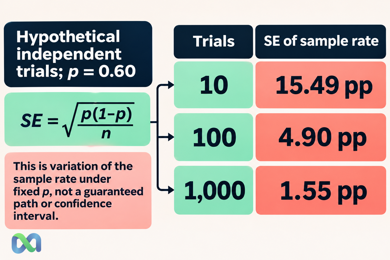
For n independent trials, the sample success rate is the number of successes divided by n. Its standard deviation, often called the standard error of the sample proportion under the model, is:
SE = √[p(1 − p) ÷ n]
The Naval Postgraduate School probability text gives the Bernoulli moments and independent-sum relationship from which this expression follows.
For the hypothetical p = 0.60 model:
| Trials | Mean count | SE |
|---|---|---|
| 10 | 6 | 15.49 pp |
| 100 | 60 | 4.90 pp |
| 1,000 | 600 | 1.55 pp |
“pp” means percentage points. The table describes the variation of the success rate across repeated samples under the model. It is not a confidence interval around an observed rate and is not a guarantee for any one sequence.
Why 10 times the data is not 10 times the precision
Standard error falls in proportion to 1/√n in this setup. Multiplying the sample size by four halves it. Multiplying by 10 reduces it by a factor of about 3.162.
For example, 100 trials have standard error of roughly 4.90 percentage points. At 400 trials it is about 2.45 percentage points. This improvement depends on the independent, common-probability model.
The standard deviation of the total success count behaves differently: √[np(1 − p)]. It grows with √n. Dividing the count by n is what makes the sample rate's variation shrink.
What the Law Means for Expected Trading Results
Consider a hypothetical contract paying $1 on success and $0 otherwise. Assume a success probability of 0.60, an entry price of $0.55, and a fixed additional cost of $0.01 per contract.
Profit per trial is $0.44 on success and −$0.56 on failure. Its expected value is:
0.60 × $0.44 + 0.40 × (−$0.56) = $0.04
If repetitions genuinely satisfy the model, the average profit per contract converges to $0.04. The expected value guide explains why that average is different from the result of any individual position.
The example assumes fixed dollar stakes, unchanged probabilities and costs, independent outcomes, and settlement according to the teaching payoff. Actual contract terms and portfolio conditions need separate analysis.
A numerical expectation is not a practical guarantee
At 100 such trials, expected total profit is $4. The total profit standard deviation is √(100 × 0.24), or about $4.90, because subtracting the fixed $0.56 cost from a zero-or-one payout does not change variance.
An expected profit of $4 therefore does not imply that a 100-trial result will be close to $4. Finite-sample losses remain possible. A long-run convergence statement does not provide unlimited capital to survive an unfavorable path.
Changing position sizes also changes the calculation. An average of equal-stake trial profits is not automatically the same as compounded account growth or a strategy that increases exposure after losses.
More negative-expectation trials do not help
Keep the all-in cost at $0.56 but change the hypothetical success probability to 0.50. Expected profit becomes −$0.06 per contract.
Under the repeated-trial assumptions, the average moves toward that negative expectation. More observations can make the average more stable around an unfavorable value. The theorem supplies no edge and does not validate the probability forecast.
This is why a high activity level, a long trading record, or a familiar success rate cannot by itself establish profitability.
Dependence and Changing Conditions
Suppose you buy 100 units of the same binary contract. The units settle together. Their outcomes are not 100 independent observations of the event.
If the common outcome has probability 0.60, the average zero-or-one payout across those identical units is still either zero or one. Its standard deviation stays √0.24, about 0.490, rather than shrinking by a factor of 10.
This constructed example shows why quantity is not statistical breadth. Positions on distinct but related events can also share dependence, although the relationship may be less extreme.
Stable assumptions need evidence
Probabilities can change with information, and strategies can change their selection criteria. Costs, market liquidity, and the set of available events can also change. A record drawn from several regimes need not resemble repeated draws from one stable distribution.
For Macro Markets readers, define the forecast question and settlement rule before collecting results. A large collection of unrelated screenshots is not necessarily a coherent sample of comparable decisions.
The conditional probability guide addresses updating probabilities when information changes. Such updates should be recorded rather than hidden inside a fixed-p trial model.
Law of Large Numbers vs Central Limit Theorem
The law of large numbers concerns where an average converges. A central limit theorem concerns the limiting distribution of an appropriately standardized sum or average under its own assumptions.
The MIT central limit theorem lecture treats that separate result. A normal approximation can help answer some finite-sample questions, but it requires checking whether the approximation is appropriate.
Neither theorem says that individual outcomes become normally distributed. A binary event remains binary regardless of how many similar trials you study.
If a question needs the exact probability of a certain number of independent successes, use an appropriate count distribution rather than invoking “large numbers” without a calculation.
How to Review a Claimed Long-Run Edge
Write down the outcome, fixed exposure unit, expected payoff, and costs. Then identify why the observations should be comparable and what could make them dependent. Keep the full record, including losses, missing observations, and changes to the selection rule.
Separate a forecast probability from an observed success rate. Estimating p from the same sample adds uncertainty. A favorable historical average can arise by chance or through selection and does not prove the future mean.
Finally, assess the account's path and constraints. Our maximum drawdown guide covers losses from earlier portfolio peaks. Convergence of an average does not report drawdown, liquidity needs, or the chance of exhausting available capital.
Frequently Asked Questions
Does the law of large numbers guarantee a profit?
No. It describes convergence toward an expected value under specified assumptions. That expected value can be negative, zero, or positive, and finite-sample losses remain possible even with a positive mean.
How many trials are enough?
There is no universal threshold. The answer depends on the model, dependence, variability, desired tolerance, and the question being asked. “Large” is not a substitute for a precision or probability calculation.
Must an average get closer after every trial?
No. The running average can move farther away after a new observation. Convergence is a statement about the sequence's limiting behavior, not a monotonic path.
Is a result due after a losing streak?
Not under an unchanged independent-trial model. A streak does not create a compensating probability. Evidence about the event or the model may justify an update, but the need to recover losses does not.
