


Standard Deviation: Formula and Portfolio Risk
Standard deviation measures how spread out values are around their mean. It is the square root of variance, so it is expressed in the same units as the original observations.
For financial returns, a standard deviation is often called volatility. It summarizes variation, but it does not tell you the maximum loss, the probability of a loss, or whether a particular investment is attractively priced.
This guide calculates population and sample standard deviation from four hypothetical monthly returns. It also explains percentage units, annualization, the difference from standard error, and the limits of using volatility for prediction market positions.
What Does Standard Deviation Mean?
Values close to their mean produce a smaller standard deviation than widely scattered values, all else equal. A constant series has a standard deviation of zero.
The calculation squares deviations, averages them using the appropriate convention, and then takes a square root. Squaring gives unusually large deviations more influence than small ones.
The NIST measures-of-scale guide explains that the square root restores the original units. If observations are dollars, standard deviation is in dollars. If observations are percentage-point returns, it is in percentage points.
It measures spread on both sides
An observation far above the mean increases standard deviation, as does one far below it. The measure does not distinguish a favorable surprise from an unfavorable one of the same size relative to the mean.
That makes it useful as a broad variability measure, while limiting what it says about downside risk. A strategy with rare large losses and one with symmetric movements can require more information than a single volatility figure.
Also identify the variable. The standard deviation of prices, simple returns, log returns, and portfolio dollar profits are different quantities. A label such as “volatility 10%” is incomplete without its horizon and methodology.
Population and Sample Standard Deviation Formulas
For a complete population of N equally weighted observations:
Population SD, σ = √{sum[(x − μ)²] ÷ N}
For a sample of n observations using the conventional sample calculation:
Sample SD, s = √{sum[(x − x̄)²] ÷ (n − 1)}
The population mean is μ and the sample mean is x̄. The sample version needs at least two observations.
Why there are two divisors
When estimating a population's variance from an independent sample, the mean is itself estimated from that sample. Dividing squared deviations by n − 1 corrects the conventional variance estimator's bias under the relevant assumptions.
Taking its square root gives sample standard deviation. The square root does not preserve unbiasedness, so it is imprecise to say this automatically makes sample SD an unbiased estimator of population SD.
The distinction is about the calculation's purpose. Describing a complete set of values and estimating a wider distribution from a sample are different tasks. Record which convention applies rather than switching between them to get a preferred number.
How to Calculate Standard Deviation
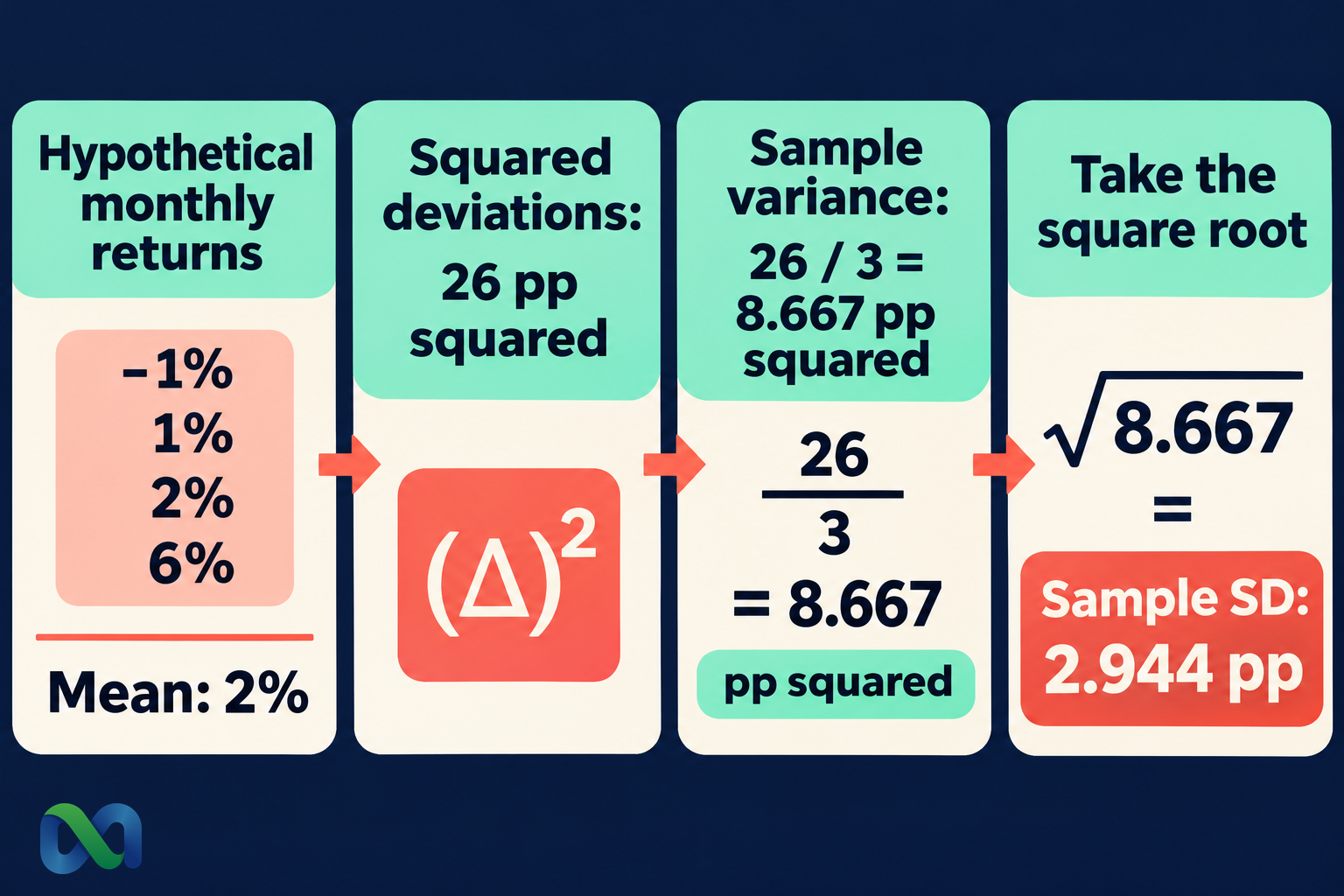
Assume four hypothetical monthly returns: −1%, 1%, 2%, and 6%. Their arithmetic mean is:
(−1 + 1 + 2 + 6) ÷ 4 = 2%
Use percentage-point numbers for the following working table. Gap means deviation from the 2% mean:
| Return | Gap | Gap² |
|---|---|---|
| −1% | −3 pp | 9 pp² |
| 1% | −1 pp | 1 pp² |
| 2% | 0 pp | 0 pp² |
| 6% | 4 pp | 16 pp² |
The squared deviations sum to 26 pp². “pp” means percentage points.
Population calculation
If those four equally weighted values are the complete population being described:
Population variance = 26 ÷ 4 = 6.5 pp²
Population SD = √6.5 ≈ 2.550 pp
The square root is essential. A variance of 6.5 pp² is not a standard deviation of 6.5%.
Sample calculation
If the four observations are a sample used to estimate a wider return distribution:
Sample variance = 26 ÷ 3 ≈ 8.667 pp²
Sample SD = √8.667 ≈ 2.944 pp
The different result comes from the divisor, not different underlying returns. Four observations are enough for an arithmetic illustration, but are not presented as a reliable real-world volatility estimate.
Percentages, Decimals, and Interpretation
The same returns in decimals are −0.01, 0.01, 0.02, and 0.06. Calculating sample SD directly from those numbers gives approximately 0.029439.
That is equivalent to 2.944 percentage points of return variation. In financial reporting it is commonly expressed as about 2.94% monthly volatility, with the monthly frequency stated.
If you instead enter the numbers −1, 1, 2, and 6, the resulting SD is about 2.944. Formatting that number as an ordinary spreadsheet percentage would show about 294.4%, which misrepresents the original inputs.
Standard deviation is not a guaranteed range
The hypothetical mean is 2%. Adding and subtracting one sample SD gives roughly −0.944% to 4.944%. The calculation alone does not assign a particular probability to that range.
For a true normal model, specific coverage percentages apply around the distribution's mean. Without that assumption, you cannot automatically say that 68% of future returns lie within one SD or 95% within two.
An estimate from a short sample also introduces parameter uncertainty. A historical range constructed from estimated mean and SD is not automatically a confidence interval or a forecast interval.
Annualizing Monthly Volatility
The familiar conversion is:
Annualized SD = monthly SD × √12
For the sample example, that gives:
2.944 pp × √12 ≈ 10.198 pp
This is a model-based annualization, not an observed full year of returns. Four monthly observations do not become 12 measured observations by changing the displayed unit.
When square-root scaling applies
Variance of a sum includes each period's variance and the cross-period covariance terms. With equal periodic variance and zero cross-period covariance, the variance of that sum is m times the periodic variance; its SD scales by √m.
Compounded simple returns are not exactly a sum of simple returns. Dependence, overlapping returns, and changing volatility can also invalidate the simple conversion. State the return definition and aggregation assumptions.
The CFA Institute market-risk discussion emphasizes that model choices affect risk estimates. A familiar scaling convention should not replace a model appropriate to the horizon and exposure.
Standard Deviation vs Standard Error
Standard deviation describes spread in the observations or underlying distribution. Standard error describes uncertainty in an estimator, such as the sample mean.
For an independent, identically distributed sample with finite variance, the estimated standard error of the mean is commonly:
SE of mean = sample SD ÷ √n
For the four-return example, that gives 2.944 ÷ √4 ≈ 1.472 percentage points. The number is smaller because it addresses the sample average rather than the spread of individual monthly returns.
The MIT lecture on the weak law of large numbers provides the probability framework for averages becoming more concentrated under suitable assumptions.
More data does not make individual returns less variable
Increasing sample size can reduce uncertainty in an estimated average under a stable model. It does not, by itself, reduce the underlying distribution's standard deviation.
If observations are dependent, s/√n may understate or otherwise misstate the mean's uncertainty. Treating many repeated marks of one exposure as independent observations is particularly problematic.
Neither an SD nor an SE becomes a confidence interval until a suitable sampling method and coverage procedure are specified.
Financial Risk Beyond Volatility
The Sharpe ratio uses variation in excess returns to relate return and risk. The Sortino ratio focuses on downside deviations relative to a specified target.
Maximum drawdown describes a fall from an earlier portfolio peak. Reordering a fixed set of returns leaves its SD unchanged but can change the drawdown path.
These distinctions matter because two datasets can have the same standard deviation and different downside shapes or sequences. Standard deviation does not identify which observation was the worst, how long a loss lasted, or how readily an exposure could be exited.
Binary settlement and interim marks
A single event indicator with probability p has SD √[p(1 − p)]. A financial payoff based on that indicator needs the appropriate payout scale and costs before interpreting dollar or percentage risk.
Historical contract price changes are a different variable from final zero-or-one settlement. Displayed values may also differ from executable prices. Define the observations before describing their SD as portfolio volatility.
For Macro Markets readers, this is an analytic framework, not a claim that the platform provides a particular volatility statistic. Start with each outcome's rules, your exposure, and the measurement horizon.
Spreadsheet Calculation and Quality Checks
In Excel, =STDEV.P(A2:A5) calculates population SD for the example range, while =STDEV.S(A2:A5) calculates sample SD.
If cells contain actual percentages such as −1%, the result is in decimal return units and can be displayed as a percentage. Keep the numeric representation consistent across all observations.
Check missing dates and duplicate rows. A missing observation is not automatically a zero return. Verify the treatment of cash flows, fees, settlement values, and stale marks before summarizing the series.
Report sample size, observation frequency, date range, divisor convention, and any annualization. Those details make the figure reproducible and clarify what it can support.
Frequently Asked Questions
Is a low standard deviation always good?
It indicates less spread in the specified observations or model. It does not establish attractive returns, adequate liquidity, a correct valuation, or the absence of rare losses.
Can standard deviation be negative?
No. It is a nonnegative square root. A negative reported value indicates a calculation or labeling problem.
Is standard deviation the average absolute distance from the mean?
No. It takes the square root of an average of squared deviations, using the stated convention. Average absolute deviation is a different measure.
Does volatility require normally distributed returns?
The SD calculation does not require normality when the variance exists. Normality is needed for specific normal-model probability interpretations, not for computing the statistic itself.
