


Correlation Coefficient: Formula and Portfolio Examples
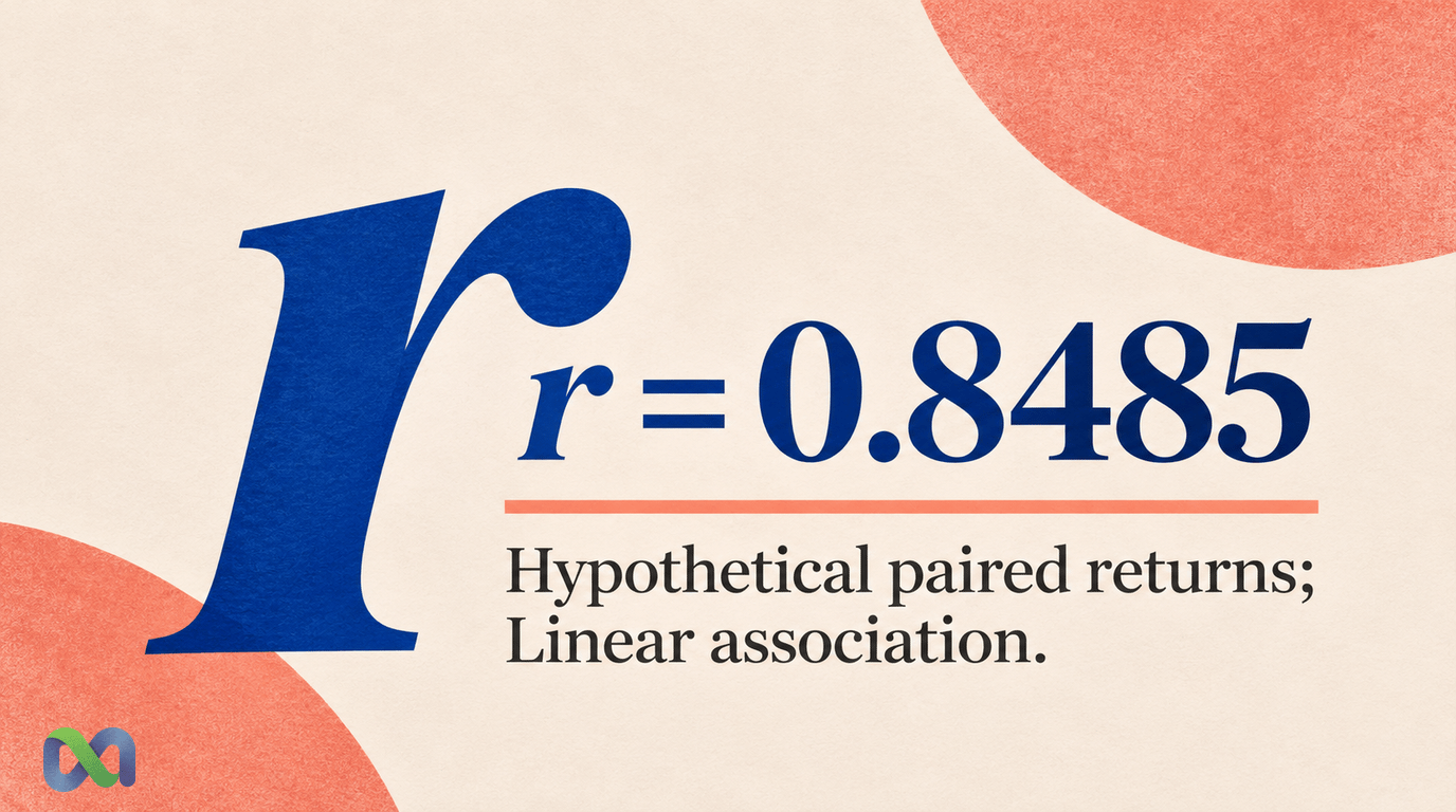
A correlation coefficient measures how two variables move together. The most familiar version, Pearson's r, summarizes their linear relationship on a scale from −1 to +1.
In a portfolio, correlation helps explain why combining two exposures can produce a different level of risk from simply averaging their individual volatility. It does not prove that one variable causes another, or that a historical relationship will persist.
This guide calculates Pearson correlation from a small dataset, applies correlation to a two-asset portfolio, and separates return correlation from dependence between binary outcomes. Every dataset and portfolio input below is hypothetical.
What Does a Correlation Coefficient Measure?
Pearson correlation compares deviations from each variable's own average. If above-average observations in one series tend to align with above-average observations in the other, the coefficient is positive. If they align with below-average observations, it is negative.
A value of +1 means an exact positive linear relationship in the observations. A value of −1 means an exact negative linear relationship. A value of zero means no linear association as measured by this coefficient.
The NIST correlation reference gives the centered-sum formula used below. Correlation has no units, which makes its numerical scale different from covariance.
There is no universal “strong” cutoff
The importance of a coefficient depends on the question, sample, measurement error, and economic exposure. A fixed label such as “strong above 0.7” is a convention, not a law of portfolio construction.
Plot the paired observations before relying on the number. A single unusual observation, a curved relationship, or a mixture of different regimes can make a one-number summary misleading.
Also state what is being correlated. Daily returns, price levels, changes in displayed probabilities, and final event indicators are different variables. They need not have the same coefficient.
The Correlation Coefficient Formula
For paired observations x and y, calculate each series' average, written x̄ and ȳ. Then calculate:
Sxx = sum[(x − x̄)²]
Syy = sum[(y − ȳ)²]
Sxy = sum[(x − x̄) × (y − ȳ)]
Pearson correlation is:
r = Sxy ÷ √(Sxx × Syy)
An equivalent expression is sample covariance divided by the product of the two sample standard deviations. The common n − 1 factors cancel when all inputs use the same paired observations and sample convention.
You need variation in both series. If one is constant, its centered sum of squares is zero and Pearson correlation is undefined. A spreadsheet error in that situation should not be replaced with zero, which would make a different claim.
The pairing matters just as much as the formula. Align the dates, time zones, return horizons, and treatment of missing observations before calculating. Pairing Monday's return in one series with Tuesday's return in the other changes the question.
Worked Example: Four Paired Returns
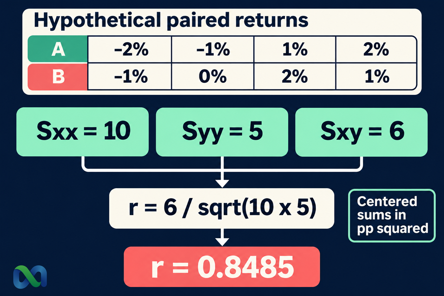
Assume these four hypothetical one-period returns:
| Period | Series A | Series B |
|---|---|---|
| 1 | −2% | −1% |
| 2 | −1% | 0% |
| 3 | 1% | 2% |
| 4 | 2% | 1% |
Use percentage-point numbers for the arithmetic. The mean of A is 0, and the mean of B is 0.5.
The deviations for A are −2, −1, 1, and 2. Their squared sum is Sxx = 10. The deviations for B are −1.5, −0.5, 1.5, and 0.5. Their squared sum is Syy = 5.
The paired deviation products are 3, 0.5, 1.5, and 1. Their sum is Sxy = 6.
r = 6 ÷ √(10 × 5) ≈ 0.8485
Using decimal returns instead produces the same coefficient because the scale factors cancel. It changes the numerical covariance, but not correlation.
Interpret the result in context
The coefficient describes a positive linear association in these four constructed observations. It does not estimate future correlation reliably from four periods, establish a causal mechanism, or prove that the two series are independent investments.
For example, both might respond to the same news. One might also be a delayed mark of a similar exposure. The coefficient alone cannot distinguish those explanations.
In Excel, =CORREL(A2:A5, B2:B5) calculates Pearson correlation for the paired ranges. Verify the raw pairs and their count rather than assuming equal-length spreadsheet columns represent synchronized observations.
How Correlation Changes Portfolio Risk
For a two-asset portfolio with fixed starting weights over the measured period:
Portfolio variance = wA²σA² + wB²σB² + 2wAwBρσAσB
Here, w represents portfolio weights, σ represents each asset's standard deviation, and ρ is their return correlation. All inputs must use the same return horizon and units.
This is a variance identity for the weighted return, not a normal-distribution assumption. The CFA Institute portfolio mathematics material treats variance, covariance, and correlation together in portfolio analysis.
Assume a hypothetical 50/50 portfolio, annual standard deviations of 10% and 20%, and correlation of 0.30. Using decimal units:
Variance = 0.5² × 0.10² + 0.5² × 0.20² + 2 × 0.5 × 0.5 × 0.30 × 0.10 × 0.20
= 0.0025 + 0.0100 + 0.0030 = 0.0155
Taking the square root gives portfolio standard deviation of approximately 12.45%.
Change only the correlation assumption
Keeping weights and individual standard deviations unchanged produces:
| Correlation | Portfolio SD |
|---|---|
| −1.00 | 5.00% |
| 0.00 | 11.18% |
| 0.30 | 12.45% |
| 1.00 | 15.00% |
These are model comparisons, not attainable forecasts or recommendations. Even perfect negative correlation does not cancel all variation with these weights because the assets have different standard deviations.
The calculation demonstrates why averaging the individual standard deviations is generally insufficient. That average equals the result at +1 correlation for this long-only example, but not at the other assumed correlations.
Correlation Is Not Independence or Causation
Zero Pearson correlation can coexist with a deterministic nonlinear relationship. Take the equally weighted values X = −1, 0, 1 and define Y = X². The paired Y values are 1, 0, 1.
The covariance is zero by symmetry, so Pearson correlation is zero. Yet knowing X tells you Y exactly. The variables are dependent despite their zero linear correlation.
Independence implies zero correlation when the relevant finite moments exist and the variances are nonzero. The reverse implication does not hold in general. Our independent events guide explains independence through joint probabilities rather than a visual resemblance between charts.
Correlation also cannot establish causation. Two series can share a driver, follow a common trend, or align by chance in a selected sample. A persuasive explanation requires evidence about the mechanism and the data-generating process.
Binary Outcomes and Prediction Market Portfolios
For event indicators A and B coded as zero or one, the covariance is:
Cov(A, B) = P(A and B) − P(A)P(B)
Divide by the product of their Bernoulli standard deviations to obtain their correlation, provided neither outcome is certain.
Suppose P(A) = 0.60, P(B) = 0.50, and P(A and B) = 0.40. The independent joint probability would be 0.30. In the stated model, covariance is 0.10 and correlation is:
0.10 ÷ √(0.60 × 0.40 × 0.50 × 0.50) ≈ 0.4082
These are assumed joint probabilities. The two separate marginal probabilities alone would not identify the joint probability or correlation.
Outcome dependence is not marked-return correlation
Historical changes in contract prices are not the same observations as final zero-or-one settlements. A coefficient computed from price returns answers a different question from the indicator calculation above.
Positions on related outcomes may share resolution rules, information, or an economic driver. A portfolio model should preserve those relationships instead of treating every displayed market as an independent trial.
For Macro Markets analysis, identify the exact variable, exposure, and holding horizon first. Use a tail-loss measure such as CVaR alongside correlation when the question concerns joint losses rather than average linear movement alone.
A Practical Correlation Review
Start with synchronized observations and a clear definition of returns. Document whether fees, cash flows, and stale or missing marks affect the series. Avoid mixing daily observations for one exposure with weekly observations for another.
Inspect a scatterplot and consider whether the relationship changes across periods. One full-sample coefficient can conceal differences between calm and stressed conditions. Re-estimate a model when the economic relationship or measurement process changes.
Distinguish Pearson correlation from rank-based measures such as Spearman correlation. Rank correlation can address a different aspect of association, but it still does not establish causation or make future relationships certain.
Finally, connect the estimate to the decision. A coefficient is one input to a portfolio model, not a complete measure of liquidity, settlement risk, expected return, or maximum possible loss. The Sharpe ratio addresses a separate comparison between excess return and its variation.
Frequently Asked Questions
Can a correlation coefficient exceed one?
A correctly calculated Pearson coefficient lies between −1 and +1 when it is defined. A result outside that range indicates a calculation, numerical, or data-handling problem.
Does negative correlation mean one asset always rises when the other falls?
No. A negative coefficient summarizes a relationship across the observations. Only a coefficient of −1 describes an exact negative linear relationship in that dataset, and even that does not guarantee the next observation.
Is correlation the same as covariance?
No. Covariance retains the product of the variables' units. Correlation divides covariance by their standard deviations, producing a unit-free number on a bounded scale.
Is zero correlation enough for diversification?
It can reduce modeled variance relative to an otherwise comparable positively correlated combination. It does not remove each exposure's risk, establish independence, or account for every feature of joint losses.
