


Exponential Distribution: Formula and Waiting-Time Examples

An exponential distribution models a nonnegative waiting time with a constant hazard rate. Its main parameter is often a rate λ, measured per unit of time. Under the rate convention, the mean waiting time is 1/λ.
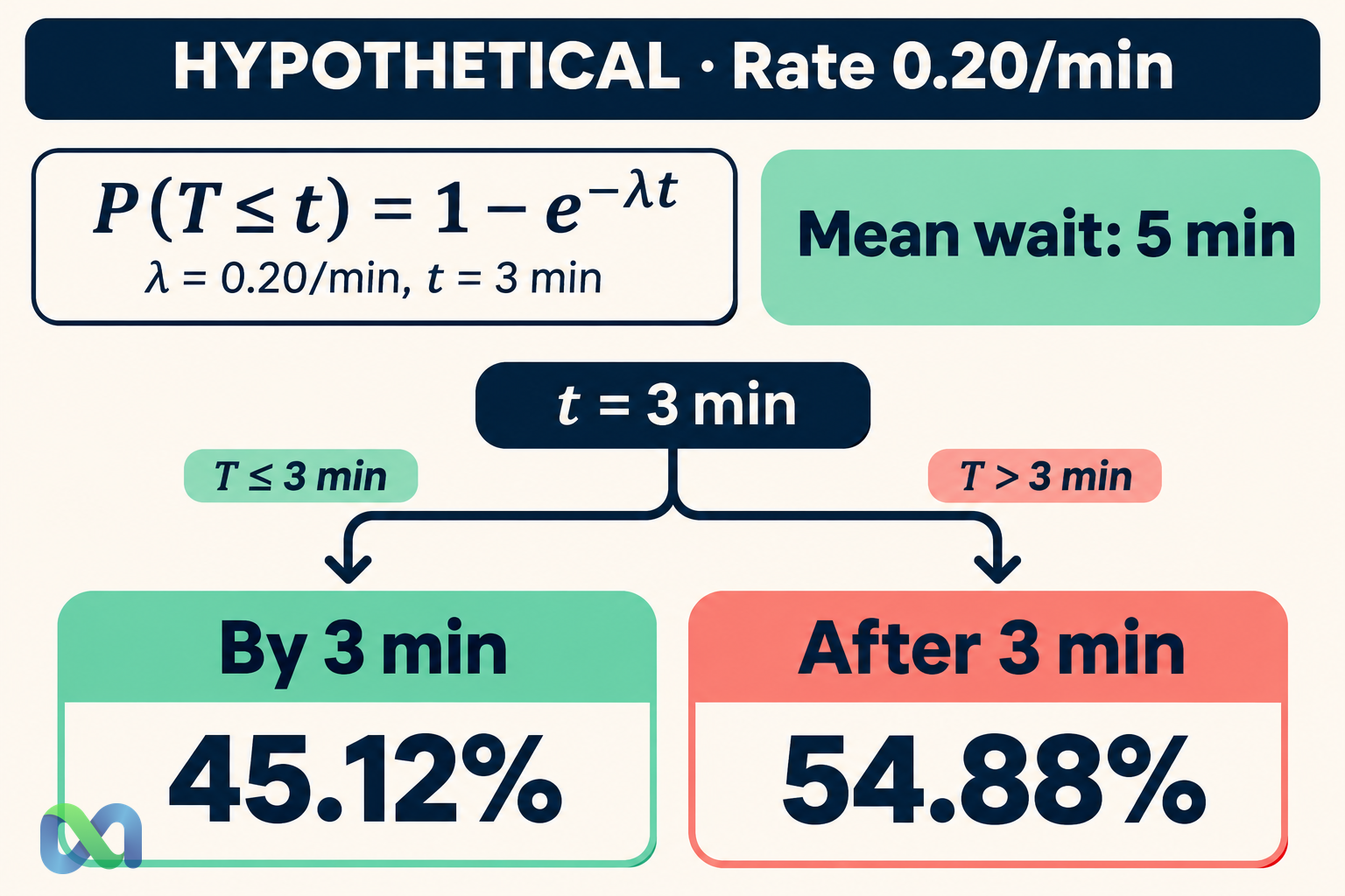
For a hypothetical event-arrival rate of 0.20 per minute, the mean wait is five minutes. The model gives a 45.12% probability of an arrival within three minutes and a 54.88% probability of waiting longer. These are model calculations, not observed arrival times or service guarantees for a trading platform.
The distribution is closely connected to Poisson counts, but the questions differ: a Poisson variable counts arrivals during a period; an exponential variable measures a wait between arrivals in the corresponding homogeneous Poisson process. This guide works through the formulas, unit conversions, and memoryless assumption.
What Is an Exponential Distribution?
Write T ~ Exponential(λ) for a waiting time T with rate λ > 0. The support is t ≥ 0. Its density declines from a maximum at zero, so short waits occupy more probability per unit of time than equally wide intervals much farther to the right.
The distribution has a long right tail and no finite upper limit. A five-minute mean does not mean an arrival happens every five minutes or that all waits are near five minutes. Occasional much longer waits are part of the model.
NIST’s exponential-model reference gives the rate-parameter formulas and explains the constant hazard. The hazard describes the instantaneous event rate conditional on having waited until that time. It is not a probability assigned to an entire minute without further calculation.
This model has specific assumptions. A scheduled announcement, a daily opening auction, or an event whose likelihood changes sharply near a deadline is not naturally described by a constant-rate exponential wait merely because it takes place in the future.
Exponential Distribution Formulas
For rate λ and time t ≥ 0, the probability density is:
f(t) = λe^(−λt)
The cumulative probability of an arrival by time t is:
P(T ≤ t) = 1 − e^(−λt)
The survival probability, meaning the chance that the wait exceeds t, is:
P(T > t) = e^(−λt)
For an interval from a to b, with 0 ≤ a < b, subtract cumulative probabilities or survival probabilities:
P(a < T ≤ b) = e^(−λa) − e^(−λb)
The density is not the probability of an arrival at one exact instant. In this continuous model, that point probability is zero. Probabilities correspond to intervals of time, and those probabilities must remain between zero and one.
Keep units consistent in λt. A rate per minute must multiply a time measured in minutes. Converting only one input can produce a plausible-looking answer to a completely different waiting-time question.
Worked Example: An Arrival Rate of 0.20 per Minute
Assume hypothetical arrivals follow a homogeneous Poisson process at λ = 0.20 per minute. The time to the next arrival follows the associated exponential model. The mean wait is:
1/λ = 1/0.20 = 5 minutes
For an arrival within three minutes:
P(T ≤ 3) = 1 − e^(−0.20 × 3) = 1 − e^(−0.60) ≈ 45.12%
For a wait longer than three minutes, take the complement:
P(T > 3) = e^(−0.60) ≈ 54.88%
The two probabilities add to one before rounding. The threshold is three minutes in both expressions; changing it from “within three” to “after three” changes the event being measured.
| t (min) | By t | After t |
|---|---|---|
| 1 | 18.13% | 81.87% |
| 3 | 45.12% | 54.88% |
| 5 | 63.21% | 36.79% |
| 10 | 86.47% | 13.53% |
An arrival by the five-minute mean is more likely than a wait beyond it. A right-skewed distribution need not put half its probability on either side of its mean.
An interval probability
The probability that the wait is longer than three minutes but no longer than eight is:
e^(−0.20 × 3) − e^(−0.20 × 8) ≈ 34.69%
This is different from the probability of an arrival within five minutes, even though the interval spans five minutes. The first question conditions on no event only implicitly through the unconditional survival difference; it starts its interval three minutes after the original clock begins.
Mean, Median, Variance, and Percentiles
For an exponential variable with rate λ, the mean and standard deviation are both 1/λ. The variance is 1/λ². At λ = 0.20 per minute, the mean and standard deviation are five minutes, and the variance is 25 minutes squared.
The median is ln(2)/λ, or approximately 3.47 minutes in this example. Half the modeled waits are shorter and half are longer. The median is below the mean because long waits pull the average upward.
The quantile at cumulative probability q is −ln(1 − q)/λ. The 95th percentile here is approximately 14.98 minutes. A five-minute average can therefore coexist with a substantial upper-tail threshold.
The standard deviation guide explains dispersion in the original units. A percentile describes a point in this modeled waiting-time distribution; it is not a confidence interval for an unknown rate and does not account for uncertainty in estimating λ.
What Memorylessness Means
The exponential distribution satisfies:
P(T > s + t given T > s) = P(T > t)
Under a fixed-rate model, knowing that an arrival has not occurred during the first s minutes does not change the distribution of the additional wait. This is a property of the model, not a claim that real systems forget their history.
In the hypothetical five-minute-mean model, the probability of an arrival in the next five minutes is 63.21%. If no arrival has occurred for 10 minutes, the conditional probability of an arrival during the following five minutes is still 63.21%, assuming the same constant rate remains valid.
The expected additional wait is still five minutes. The elapsed 10 minutes do not reduce the remaining expected wait to a negative value or make an arrival overdue. They also do not prove the rate assumption is correct.
If inactivity provides information about a hidden state, such as a closed session or failed connection, the conditional distribution may change. That is evidence that a single fixed-rate exponential model may be inadequate for the actual process.
Exponential vs. Poisson Distribution
The Poisson distribution models counts over a specified interval. In a homogeneous Poisson process with rate λ, the count over duration t has mean λt, while successive interarrival times are independent exponential variables with mean 1/λ.
For the example rate, the expected count over 10 minutes is two. The probability of zero arrivals during that period is e^(−2) ≈ 13.53%. That matches the probability that the first wait exceeds 10 minutes.
This correspondence depends on the process assumptions, including a constant rate and independent increments. A count distribution fitted over a particular period does not by itself prove that all interarrival times are independent exponential draws. Clustering and time-varying intensity can break that relationship.
Keep the parameters distinct. “Two arrivals expected over 10 minutes” is an expected count. “0.20 arrivals per minute” is a rate. “Five minutes” is a mean wait. Their units help identify which formula belongs to the question.
Rate vs. Scale: A Common Parameter Mistake
Some references and software use a scale β = 1/λ. The density then becomes (1/β)e^(−t/β) for t ≥ 0. A five-minute scale and a 0.20-per-minute rate describe the same unshifted exponential model.
NIST’s distribution gallery presents the scale formulation and also discusses a location parameter. The location-shifted form is a different specification from the zero-start model used throughout this example.
Do not enter five as the rate when the intended mean wait is five minutes. A rate of five per minute would imply a mean wait of 0.20 minutes, or 12 seconds. Reversing rate and scale can change the answer dramatically while leaving the software calculation valid.
In an English-language spreadsheet, the cumulative probability for three minutes at rate 0.20 is =EXPON.DIST(3,0.2,TRUE). The survival probability is =EXP(-0.2*3). Confirm the software’s parameter convention and units rather than assuming every function uses the same inputs.
When the Exponential Model Is a Poor Fit
The constant hazard can be unrealistic when arrivals cluster around economic releases, vary with trading hours, or respond to recent events. A model that averages quiet and busy periods may describe neither period well.
Waiting until a known settlement deadline is another distinct question. A contract’s resolution time can depend on official procedures, data availability, and dispute rules. It should not be described as exponential without evidence supporting that model.
The exponential distribution also has no maximum wait. If a process has a hard cutoff, the unmodified model assigns positive probability to impossible times. Truncation, censoring, and deadlines need explicit treatment.
For a simulation, document the source or rationale for λ, the time unit, and the observation window. Use the Monte Carlo guide to separate numerical simulation precision from uncertainty about whether the assumed arrival process matches reality.
Frequently Asked Questions
Does a five-minute mean mean one arrival every five minutes?
No. It is an average waiting time under the model. Individual waits vary, and some can be much longer. A fixed five-minute schedule would have a different waiting-time structure.
Does waiting longer make an arrival more likely soon?
Not under a fixed-rate exponential model: the conditional distribution of the additional wait stays the same. In a real process, changing information can alter the rate or show that the model is inappropriate.
Can this distribution predict a financial event by itself?
It can calculate waiting-time probabilities after a suitable model and rate have been specified. It does not independently establish the rate, validate a forecast, or determine a contract’s expected value at an available price.
