


Monte Carlo Simulation: Portfolio Risk Examples

A Monte Carlo simulation repeatedly samples outcomes from a specified probability model and calculates what those outcomes imply. In portfolio analysis, it can estimate quantities such as average profit, loss probability, or a loss quantile.
The simulation does not discover the correct probabilities by itself. Its results depend on the payoff rules, distributions, dependence, costs, and horizon supplied to the model.
This guide builds a reproducible simulation for two hypothetical binary positions, checks it against an exact calculation, and changes the dependence assumption. The example uses teaching inputs and is not a backtest, market forecast, or actual platform performance.
What Is a Monte Carlo Simulation?
Monte Carlo is a computational method: generate random samples, apply a calculation to each sample, and summarize the results. Repeating the procedure approximates properties of the chosen model.
For a portfolio, one simulated scenario might specify which events occur or how several risk factors change. A payoff function converts those sampled outcomes into portfolio value or profit.
The CFA Institute market-risk material identifies Monte Carlo simulation as one approach to estimating portfolio risk. It requires specifying a distribution and generating outcomes from it; flexibility does not remove model risk.
Simulation, backtesting, and stress testing
A simulation generates outcomes from a model. A historical backtest applies defined rules to historical data. A stress test examines deliberately chosen adverse assumptions or scenarios.
They can complement each other, but they are not interchangeable evidence. A profitable simulated average does not show that real trades could have been executed at the assumed prices.
Likewise, a scenario absent from a simulation may be omitted by the model rather than genuinely impossible. A large sample cannot generate a settlement state that the payoff model never included.
Define the Portfolio Before Sampling
Assume one hypothetical position on event A and one on event B, both evaluated at a common settlement horizon. Each pays $1 if its event occurs and $0 otherwise.
Use these teaching inputs:
| Input | Event A | Event B |
|---|---|---|
| Event probability | 60% | 40% |
| Entry cost | $0.55 | $0.35 |
| Successful payoff | $1 | $1 |
Add a fixed $0.02 total cost for the two-position portfolio. The all-in outlay is therefore $0.92. Initially assume that A and B are independent.
These are generic payoff terms, not a description of a specific Macro Markets product. Actual fees, payoff units, settlement exceptions, and available prices require separate verification.
Write the payoff equation
Let A and B be zero-or-one occurrence indicators. Then:
Portfolio profit = A + B − $0.92
Possible profits are −$0.92, $0.08, and $1.08. A constant subtraction changes the mean but not the variance of the sampled payout.
The model stops at settlement. It does not describe executable early exits, interim marks, cash flows, or the account's drawdown path. Those questions would require additional inputs and, in some cases, simulated paths rather than terminal outcomes alone.
Calculate the Exact Answer First
With only two binary positions, all four joint outcomes can be enumerated. Under independence:
P(A = 1, B = 1) = 0.60 × 0.40 = 0.24
The two single-success outcomes have probabilities 0.60 × 0.60 = 0.36 and 0.40 × 0.40 = 0.16. Neither event occurs with probability 0.40 × 0.60 = 0.24.
Group those outcomes by their resulting profit:
| Profit | Probability |
|---|---|
| −$0.92 | 24% |
| $0.08 | 52% |
| $1.08 | 24% |
The probabilities sum to one. Expected profit is:
−$0.92 × 0.24 + $0.08 × 0.52 + $1.08 × 0.24 = $0.08
The probability of a positive profit is 76%. Profit variance is 0.48 dollars squared and standard deviation is about $0.69282.
The expected value guide explains the probability-weighted average, while the independent events guide explains the multiplication used for the joint probabilities.
Run a Reproducible Python Simulation
The following code samples 100,000 pairs of independent binary outcomes. It uses NumPy's generator with a fixed seed, so the calculation can be reproduced with the recorded environment.
import numpy as np

rng = np.random.default_rng(20261109)
n = 100_000
probabilities = np.array([0.60, 0.40])

uniform_draws = rng.random((n, 2))
outcomes = (uniform_draws < probabilities).astype(int)
profit = outcomes.sum(axis=1) - 0.92

print(profit.mean())
print((profit > 0).mean())
print(profit.std(ddof=1))
For each column, a uniform draw below the event probability becomes one. Otherwise it becomes zero. Independent draws implement the stated independence assumption; they do not establish that real events are independent.
The NumPy random-generator documentation describes default_rng and its generator interface. Record the library version as well as the seed because reproducibility should not rely on an unstated environment.
Results from this teaching run
Running this code with NumPy 2.5.4 produced:
| Metric | Run | Exact |
|---|---|---|
| Mean profit | $0.07826 | $0.08000 |
| P(gain) | 75.838% | 76.000% |
| Profit SD | $0.69390 | $0.69282 |
Here, P(gain) means the probability of a positive profit, and Run reports the simulation result. The simulation had 24,162 zero-success scenarios, 51,850 one-success scenarios, and 23,988 two-success scenarios. Those counts sum to 100,000.
The differences from the exact model are sampling variation. A simulation need not match the theoretical probabilities exactly, even with a fixed seed and correct implementation.
More Draws Reduce Sampling Error, Not Model Error
For independent simulation draws with finite variance, the standard error of the estimated mean falls roughly as 1/√N, where N is the number of draws.
For this model, the theoretical standard error at 100,000 draws is:
√(0.48 ÷ 100,000) ≈ $0.00219
That is uncertainty from numerical sampling under the assumed model. It does not include uncertainty about the event probabilities, costs, dependence, or omitted settlement states.
Multiplying the draws by four roughly halves that sampling error. It does not make a wrong 60% forecast more accurate or convert a theoretical entry price into an executable quote.
Exact enumeration is better for this small model
For two binary positions, the exact table is simpler and more precise than simulation. The small example makes Monte Carlo's mechanics transparent and provides a reference answer against which to check the implementation.
Simulation becomes more useful when a justified model has many risk factors, complex payoffs, or path-dependent features that are difficult to enumerate. Choose the method for the problem rather than simulating solely to make the analysis look sophisticated.
Change the Dependence Assumption
Now preserve P(A) = 0.60 and P(B) = 0.40, but assume P(A and B) = 0.35 instead of 0.24.
A valid joint probability table is then 0.35 for both, 0.25 for A only, 0.05 for B only, and 0.35 for neither. These add to one and recover the stated marginal probabilities.
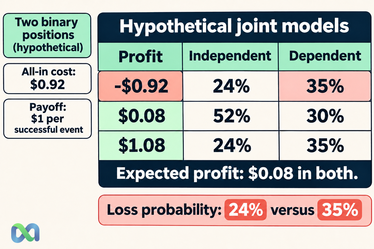
The resulting profit probabilities are shown below. Indep. denotes the independent model, and Dep. denotes the specified dependent model:
| Profit | Indep. | Dep. |
|---|---|---|
| −$0.92 | 24% | 35% |
| $0.08 | 52% | 30% |
| $1.08 | 24% | 35% |
Expected profit remains $0.08 because the individual expected payouts and fixed total cost are unchanged. However, the chance of a loss rises from 24% to 35%, and profit variance rises from 0.48 to 0.70 dollars squared.
The example demonstrates that matching marginal probabilities is not enough to specify portfolio risk. The joint model determines how often positions win or lose together.
Do not change dependence accidentally
Sampling each event independently imposes independence. Reusing the same random uniform draw for several events creates a different dependence structure. Neither choice should be made accidentally in code.
For a larger model, validate that the generated joint behavior matches the intended economic and contractual relationships. A correlation matrix alone may not capture every relevant tail relationship or logical constraint.
For Macro Markets readers, different market labels do not prove independent outcomes. Shared information, linked events, and settlement criteria can all matter to the joint payoff distribution.
Reviewing Simulation Outputs
Check units, signs, horizon, total cost, and impossible outcomes before reading the summary statistics. For the initial teaching model, simulated profit must be one of −$0.92, $0.08, or $1.08. Any other profit points to a coding or modeling mismatch.
Compare a small model with an exact calculation, and test limiting cases such as event probabilities of zero or one. Then vary substantive assumptions rather than only rerunning seeds.
If estimating conditional value at risk, state the loss convention, horizon, confidence level, and treatment of discrete probability mass at the quantile. A tail average needs enough relevant simulated observations and a clearly specified definition.
Maximum drawdown requires a portfolio value path. A histogram of settlement profits alone does not establish the worst peak-to-trough decline during the holding period.
Preserve the seed, version, model inputs, payoff logic, and output counts. That record allows another reader to reproduce the numerical experiment and distinguish it from a claim about actual market returns.
Frequently Asked Questions
Does Monte Carlo predict what will happen?
It approximates outcomes under the specified model. It does not establish the model's truth or guarantee the next realized result.
How many simulations are enough?
There is no universal count. Required precision, payoff variability, rare-event probabilities, and computational cost matter. Assess sampling error for the output being estimated and separately assess model uncertainty.
Does a fixed seed remove randomness from the model?
It makes the pseudorandom numerical sequence reproducible in the recorded setup. It does not make the hypothetical events certain or eliminate uncertainty in the model assumptions.
Can I simulate each contract separately and add the results?
You can add payoff calculations, but the simulated joint outcomes must preserve the intended dependence. Independently sampling related contracts can understate or otherwise distort portfolio risk.
