


Poisson Distribution: Formula and Event Counts

A Poisson distribution models how many events occur within a specified interval. Its parameter, λ, is the expected event count for that interval, not the probability that an event occurs.
For example, a hypothetical model with two qualifying events per hour can calculate the probability of exactly three in the next hour. It can also calculate the probability of at least one. Those answers depend on the event definition, interval, and suitability of the model.
This guide explains the Poisson distribution formula, shows the calculations, and separates event counts from binary market outcomes. The rates and examples are hypothetical; they are not observed activity or forecasts for any platform.
What Is a Poisson Distribution?
A Poisson variable counts occurrences: zero, one, two, three, and so on. Write X ~ Poisson(λ). The count has no fixed upper bound in the mathematical distribution.
The interval can be an hour, a day, a distance, or another defined amount of exposure. The units must be stated because an average of two per hour is different from two per day.
The NIST Poisson distribution reference provides its probability formula and identifies λ as the average count in the given interval. In this model, both the mean and variance equal λ.
Events do not need to be dramatic or financially significant. The counted item could be an arrival, a reported incident, or a precisely defined qualifying occurrence. Specify the counting rule before choosing a rate.
Distribution versus process assumptions
A Poisson distribution describes a count for one interval. A homogeneous Poisson process supplies a stronger model across time: a constant rate, independent counts in non-overlapping intervals, and events occurring singly in sufficiently short intervals.
The MIT Poisson-process lecture develops this process model. It motivates the rate-scaling example below. It should not be assumed simply because a dataset contains event counts. Clusters, daily cycles, and a changing environment can violate the simple model.
For example, scheduled releases are not automatically random arrivals at a constant rate. An hour around a scheduled announcement can differ from an ordinary hour. A clearly named event is necessary, but not sufficient, for a useful Poisson model.
The Poisson Distribution Formula
The probability of exactly k events is:
P(X = k) = e^(−λ) × λ^k ÷ k!
Here, e is approximately 2.71828, λ is the expected count for the selected interval, and k is a nonnegative whole number. The factorial k! multiplies the positive integers through k, with 0! defined as one.
The formula assigns a probability to an exact count. For “at most k,” add the probabilities from zero through k. For “at least k,” subtract the cumulative probability through k − 1 from one.
At λ = 0, the model puts all probability on zero events. For λ greater than zero, every nonnegative count has some probability, although very large counts can be extremely unlikely.
The distinction between exact and cumulative probabilities matters in threshold markets. “At least two” includes two; “more than two” starts at three. Always translate the contract's actual wording into the corresponding count condition.
Worked Example: Two Events per Hour
Assume a hypothetical qualifying-event process with a constant rate of two per hour. Model one hour, so λ = 2.
For exactly three events:
P(X = 3) = e^(−2) × 2³ ÷ 3!
≈ 0.135335 × 8 ÷ 6 ≈ 0.180447
The probability is approximately 18.045%. The count's expected value is two, but exactly three remains a possible outcome.
A probability table
The first five count probabilities are:
| Events | Probability |
|---|---|
| 0 | 13.534% |
| 1 | 27.067% |
| 2 | 27.067% |
| 3 | 18.045% |
| 4 | 9.022% |
These rows do not sum to 100% because five or more events remain possible. That omitted tail is about 5.265%. Truncating a table does not truncate the underlying distribution.
For this integer value of λ, one and two events are tied as the most likely individual counts. Neither has probability above 50%.
At least one and at least two
The chance of at least one event is easiest to find using the complement:
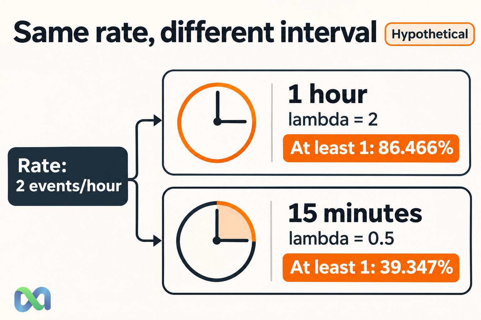
P(X ≥ 1) = 1 − P(X = 0) = 1 − e^(−2) ≈ 86.466%
For at least two, subtract the zero-event and one-event probabilities:
P(X ≥ 2) = 1 − [P(X = 0) + P(X = 1)] ≈ 59.399%
An expected count of two is therefore not a 200% chance of an event. A count expectation and a probability have different meanings and units.
Converting a Rate to the Correct Interval
Under the constant-rate process assumption, multiply the rate by the interval length in matching units:
λ = rate × exposure
At two events per hour, a 15-minute interval is one-quarter of an hour. Its expected count is therefore:
λ = 2 × 0.25 = 0.50 events
The probability of at least one event in that interval is:
1 − e^(−0.50) ≈ 39.347%
It is not one-quarter of the one-hour probability. The expected count scales linearly with exposure in this model; the probability of at least one follows the exponential formula.
Likewise, a two-hour interval has λ = 4, not λ = 2. Reusing the hourly parameter for every horizon would answer the wrong question.
When simple scaling is inappropriate
If the rate changes during the interval, a constant average may hide important structure. A nonhomogeneous Poisson process can model a deterministic time-varying intensity, but it requires an appropriate intensity function and suitable independence assumptions.
Changing intensity is also different from events causing more events. A burst triggered by an earlier occurrence introduces a dependence mechanism that a constant-rate model omits. Our independent events guide explains why separate observations do not, by themselves, establish independence. Do not fix that issue by merely changing the time unit.
Mean, Variance, and a Basic Data Check
For a Poisson count:
Mean = λ; variance = λ; standard deviation = √λ
With λ = 2, the mean is two events, the variance is two events squared, and the standard deviation is about 1.414 events. The mean and variance have the same numerical value but different units.
One preliminary diagnostic is to compare the sample mean and variance across equal-exposure intervals. A much larger variance can indicate clustering, changing rates, mixed populations, or other structure. A smaller variance can also signal a poor fit.
Equality in a small sample does not validate the model. Examine the count histogram, timing, observation window, and event definition as well. Check whether zero-event intervals are present in the dataset; omitting them biases the estimated rate upward.
If observation windows have different lengths, do not average their raw counts as though exposure were equal. Under the simple constant-rate model, total events divided by total exposure estimates the rate.
Poisson vs Binomial and Binary Outcomes
A binomial model starts with a fixed number of independent trials and a common success probability. A Poisson model starts with an expected count over an interval and permits any nonnegative whole-number count.
The two can be related. For a large number of independent opportunities with a small success probability, a binomial count can sometimes be approximated by a Poisson count with λ = np. The approximation's adequacy depends on the inputs and which probabilities matter.
Do not use it mechanically for a short list of high-probability events. When the exact binomial calculation is available, it can avoid unnecessary approximation error.
A count can define a binary event
Suppose a hypothetical contract pays $1 when at least two qualifying events occur in one hour and $0 otherwise. Under the λ = 2 model, the event probability is about 59.399%.
If the hypothetical entry price is $0.55 and all-in additional fixed cost is $0.01 per contract, modeled expected profit at settlement is:
$1 × 0.593994 − $0.55 − $0.01 ≈ $0.033994
This is a generic teaching payoff. It does not establish a real platform's contract terms or an executable opportunity. A different counting rule, rate, fee, or settlement treatment changes the analysis.
The expected value guide explains how an event probability enters a payoff calculation. The conditional probability guide explains why new information may change that probability.
For Macro Markets readers, the practical step is to separate the underlying count model from the actual binary question. A model for event arrivals is only useful when its counting rule matches the resolution criteria.
Spreadsheet Calculation and Interpretation
Using Excel’s POISSON.DIST function, exactly three events at λ = 2 is:
=POISSON.DIST(3,2, FALSE)
At least two events is:
=1-POISSON.DIST(1,2, TRUE)
The first returns about 0.180447 and the second about 0.593994. The TRUE argument requests a cumulative probability through the supplied count.
Keep full precision in intermediate calculations and round the final displayed result. For a probability table, retain an “other counts” tail or explicitly state which counts are omitted.
Record the event definition, exposure unit, assumed rate, data period if estimated, and model limitations beside the calculation. More decimal places do not compensate for a poorly justified rate or omitted dependence.
Frequently Asked Questions
Does Poisson require rare events?
The distribution is defined for any nonnegative λ. Rare events are relevant to its use as an approximation to some binomial counts, but rarity alone does not establish that a real process is Poisson.
Can λ be a decimal?
Yes. The expected count can be 0.5 or 2.7 even though an observed count is a whole number. A decimal λ is not a fractional event occurring in one observation.
Is the time between events Poisson distributed?
No. Under a homogeneous Poisson process, counts are Poisson and waiting times between successive events are exponential. These are different random variables with different units.
What if the data have too many zeros?
First check the observation and counting process. Excess zeros relative to the fitted model can reflect mixed regimes or structural zeros. Alternative count models may help, but choosing one requires evidence about the mechanism rather than a cosmetic adjustment.
