


Normal Distribution: Formula and Financial Limits
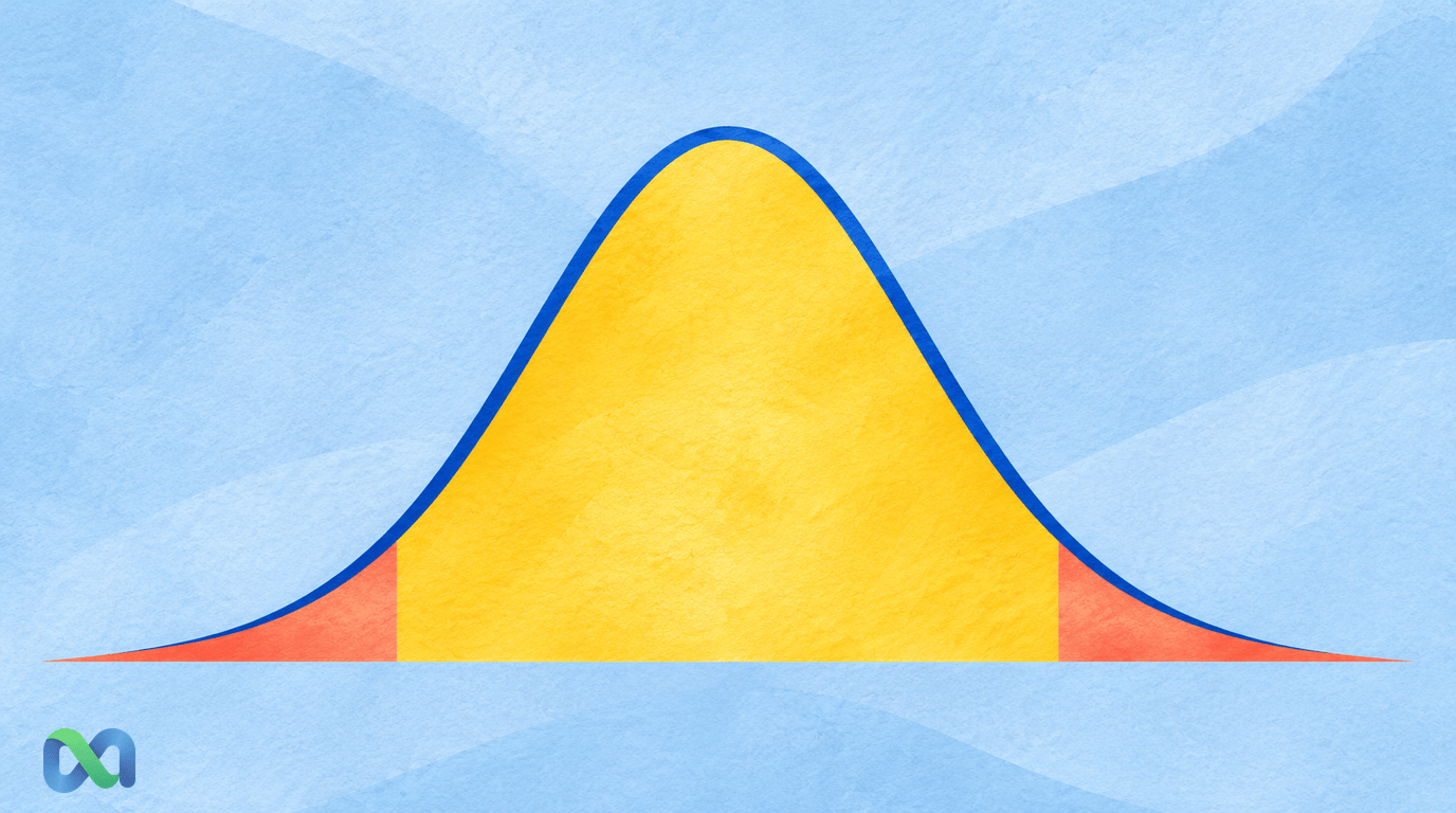
A normal distribution is a continuous, symmetric probability distribution centered on its mean. Its familiar bell shape is determined by two parameters: the mean μ and the standard deviation σ.
It is useful for many statistical calculations, including some financial models. Its convenience does not mean that every return series, event probability, or portfolio loss follows a normal distribution.
This guide explains the formula, standardization, and the 68–95–99.7 rule, then calculates probabilities for a hypothetical monthly return model. It also shows where the model can be misleading for financial and binary event outcomes.
What Is a Normal Distribution?
A normal distribution assigns probability across a continuous number line. Values near the mean have greater density than values far away, and the curve is symmetric around the mean.
Write X ~ Normal(μ, σ²), where the second parameter is the variance. State that convention because some software interfaces request standard deviation instead.
The NIST normal distribution reference gives the density and defines the standard normal case. A nondegenerate normal model has σ greater than zero and allows values anywhere on the real line.
Density is not point probability
For a continuous variable, probability is an area under the density curve over an interval. The probability of one exact value is zero, even though the density at that value can be positive.
That does not make a neighborhood around the value impossible. “Exactly 1.000000…%” and “between 0.9% and 1.1%” are different questions.
This distinction is especially important when comparing a continuous model with a binary outcome. A zero-or-one event has probability mass on two points. It is not a continuous bell curve with probability zero at each possible settlement.
The Normal Distribution Formula
The probability density is:
f(x) = exp[−(x − μ)² ÷ (2σ²)] ÷ [σ√(2π)]
The mean μ determines the curve's center. The standard deviation σ controls its spread. Increasing σ spreads the probability over a wider range and lowers the peak so the total area remains one.
You do not usually need to integrate this expression by hand. Statistical software or a spreadsheet can evaluate the cumulative distribution function, written Φ for the standard normal distribution.
Standard normal distribution and z-scores
The standard normal distribution has mean zero and standard deviation one. Transform a normal variable using:
Z = (X − μ) ÷ σ
A z-score gives the distance from the mean in standard-deviation units. Z = 1 is one standard deviation above the mean; Z = −2 is two below it.
For a normal X, P(X ≤ x) = Φ[(x − μ) ÷ σ]. For an interval from a to b, subtract the two cumulative probabilities. A z-score can be calculated for other data too, but that calculation alone does not make their distribution normal.
The 68–95–99.7 Rule
Under a normal model, approximately 68.27% of probability falls within one standard deviation of the mean, 95.45% within two, and 99.73% within three.
| Range | Coverage |
|---|---|
| Within 1 SD | 68.27% |
| Within 2 SD | 95.45% |
| Within 3 SD | 99.73% |
These percentages describe the assumed distribution. They are not universal coverage rates for arbitrary data and are not confidence intervals for an unknown mean.
For example, μ ± 2σ is a range for individual model outcomes. A confidence interval estimating μ uses a sampling framework and a measure of uncertainty in the estimated mean. Confusing the two can greatly understate or overstate uncertainty.
The tails still have probability
Even a three-standard-deviation range leaves probability outside it. The normal distribution has no finite maximum or minimum. An observation beyond that range is possible under the model.
“Three sigma” therefore does not mean impossible, and a fitted three-sigma boundary does not guarantee a future loss limit. It also says nothing about whether the fitted model adequately represents the real tails.
Worked Example: A Monthly Return Model
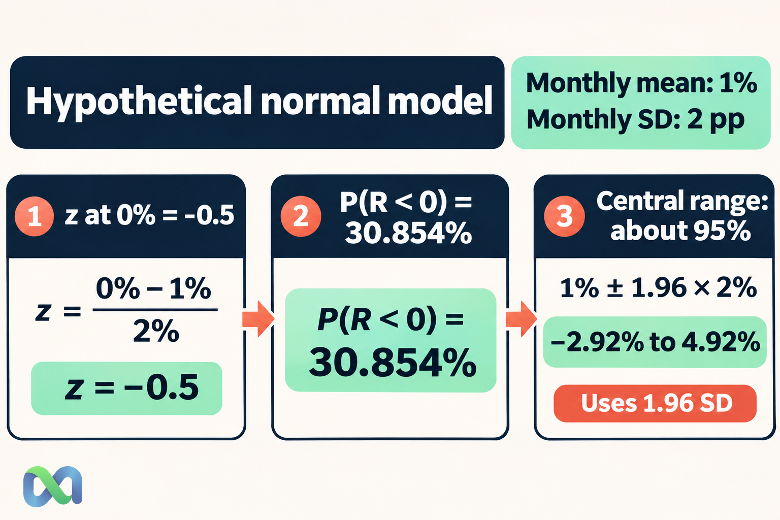
Assume a hypothetical monthly simple return R follows a normal distribution with mean 1% and standard deviation 2 percentage points. This is an assumed probability model, not a fitted record or a forecast.
In decimal notation, μ = 0.01 and σ = 0.02. To calculate the chance of a negative return, standardize zero:
z = (0 − 0.01) ÷ 0.02 = −0.5
P(R < 0) = Φ(−0.5) ≈ 30.854%
The model has a positive expected return and still assigns substantial probability to a negative month. The sign of the mean does not determine every outcome.
A range around the mean
One standard deviation around 1% runs from −1% to 3%. Under the assumed normal model, about 68.27% of returns fall inside that range.
A central range using 1.96 standard deviations runs from:
1% − 1.96 × 2% = −2.92%
to:
1% + 1.96 × 2% = 4.92%
Its model coverage is approximately 95%. The two tails together account for approximately 5%, with about half in each tail because the distribution is symmetric.
The boundaries are not predictions of the lowest and highest return that will occur. Nor is this range a 95% confidence statement about an estimated parameter; the example assumes μ and σ as inputs.
Normality, Sample Averages, and Financial Returns
The central limit theorem helps explain why normal approximations arise for some sums and averages under suitable conditions. It does not require the original individual observations to be normal in every version.
The MIT central limit theorem lecture treats this standardized-sum result. Applying it to a particular sample requires checking the relevant assumptions and approximation quality.
It does not establish that one asset's daily returns are normal or that a binary settlement becomes continuous after many observations. The random variable being approximated matters.
Financial tails can differ from a normal model
The CFA Institute market-risk material identifies limitations of normal-based risk estimates when returns are not normal. A convenient symmetric curve can miss skew, jumps, changing volatility, and dependence.
Inspect a histogram and an appropriate probability plot, and consider the mechanism behind the data. A short period without large losses is weak evidence about rare future outcomes.
Normal simple-return models also permit returns below −100%, which may be incompatible with a particular unlevered investment payoff. A normal log-return model has different implications and needs its own definition. Neither should be chosen without matching the exposure.
Limits for Prediction Market Analysis
A binary settlement indicator takes values zero and one. A normal variable permits a continuous range extending below zero and above one. Those supports are different.
Approximating some large sums of binary outcomes can be useful, but it does not make a single event normal. Dependence, small sample size, and probabilities near the boundaries can make a simple approximation poor.
A displayed probability is also bounded between zero and one. An unconstrained normal model for its future level can assign impossible values. Model the appropriate variable and enforce the relevant support rather than drawing a bell curve around a quote.
For Macro Markets readers, distinguish a forecast of event occurrence, a model of changing contract valuations, and a distribution of portfolio returns. A normal assumption for one does not automatically transfer to the others.
Compare the question with alternative risk summaries
The Sharpe ratio uses return variation but does not, by itself, prove a return distribution is normal. Its interpretation needs context when the payoff shape is asymmetric.
Conditional value at risk focuses on a selected worst tail under the stated loss model. It can be calculated for discrete or non-normal outcomes, provided their probabilities and losses are specified appropriately.
For a binary payoff, the expected value calculation combines the event forecast with its payoff and costs; it does not require a normal model of settlement outcomes.
Use an empirical or scenario-based model when it better represents the exposure. Replacing a normal curve does not eliminate the need to justify the alternative's inputs.
Spreadsheet Calculations and Review
In Excel, the hypothetical negative-return probability is:
=NORM.DIST(0,0.01,0.02, TRUE)
It returns about 0.308538. The TRUE argument requests cumulative probability; FALSE requests the density, which is a different quantity.
For the probability from −1% through 3%, subtract:
=NORM.DIST(0.03,0.01,0.02, TRUE)-NORM.DIST(-0.01,0.01,0.02, TRUE)
It returns about 0.682689. Keep all returns in the same units and pass standard deviation, not variance, as the third argument.
Before using a result, document the variable, horizon, parameters, estimation method if any, and why normality is a useful approximation. Stress the assumptions as well as recalculating the arithmetic.
Frequently Asked Questions
Is every bell-shaped distribution normal?
No. A roughly bell-shaped histogram is not enough to establish a normal distribution, particularly in its tails. Consider the data, sample size, and model diagnostics.
Are the mean, median, and mode equal?
They coincide at μ for a nondegenerate normal distribution. A finite sample drawn from that distribution need not have identical sample mean, median, and mode.
Is a z-score itself a probability?
No. It measures distance from a mean in standard-deviation units. A distributional assumption is needed to convert that distance into a probability.
Does 95% coverage guarantee 95 out of the next 100 observations?
No. It is a model probability for an individual observation in that range. A finite count varies, and the model itself may be inappropriate for the real observations.
