


Sensitivity Analysis: Methods and Financial Examples

Sensitivity analysis asks a simple question: how much does the answer change when an input changes? Start with a model, change an input, and work out the result again. The aim is to find which assumptions can change your decision. Correct math alone does not make an uncertain input correct, so it helps to look beyond one neat final number.
For a financial decision, you might test the event chance, entry price, fee, funding cost, or quantity. A small expected edge can vanish after a small change in one of those inputs. A table lets you see that weak point. It shows what follows from each input; it does not tell you which input will turn out to be right.
This guide uses a hypothetical contract payoff to test probability and price, first on their own and then together. It also shows how to repeat the math in Excel and find the break-even point. All amounts are teaching inputs. They are not current Macro Markets quotes, fees, terms, or forecasts of returns. Use actual rules and costs when building a model for a real decision.
What Is Sensitivity Analysis?
Sensitivity analysis varies inputs and observes the effect on a defined output. The output could be expected net profit, project value, a loan payment, or a funding requirement. A useful analysis states both the model and the decision it is meant to inform.
A one-way analysis changes one input while holding the others fixed. A two-way analysis evaluates pairs of input values. More complex analyses can examine interactions among many inputs, but complexity is not automatically an improvement. Start with the assumptions that could reasonably change the decision.
Microsoft's data-table documentation describes one-variable and two-variable tables as tools for what-if analysis. Those tables calculate the consequences of supplied values; they do not determine whether the supplied values are plausible.
The distinction between calculation and evidence matters. Testing a probability from 50% to 70% does not establish that the true probability lies in that range. Choose and justify the range separately from calculating its consequences.
Start With an Explicit Financial Model
Assume a hypothetical purchase of n identical contracts on one event. Each contract pays $1 if the event occurs and $0 otherwise. Let q be the purchase price per contract, p the assumed event probability, and c a fixed total extra cost paid regardless of settlement.
Under these assumptions, expected net profit is:
EV = n × (p − q) − c
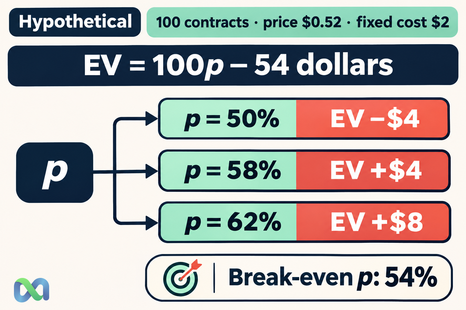
Use n = 100, q = $0.52, p = 0.58, and c = $2. The expected settlement payout is $58, purchase cost is $52, and extra cost is $2. Expected net profit is therefore $4.
The two realized settlement results are +$46 if the event occurs and −$54 otherwise. Neither is the expected value of $4. The expected value is the probability-weighted average 0.58 × $46 + 0.42 × (−$54).
This simplified cost structure is intentional. If an actual fee depends on price, quantity, or settlement, represent that dependency in the model instead of treating the fee as a constant. The expected value formula guide provides the underlying payoff framework.
One-Way Sensitivity: Change the Probability
Keep quantity, price, and extra cost fixed at their baseline values. The model reduces to:
EV = 100p − 54
Now vary p. Each one-percentage-point increase in p changes expected net profit by $1 for this 100-contract example. That is a change of 0.01 in the probability input, not a multiplication by one whole unit.
| Assumed p | Expected net |
|---|---|
| 50% | −$4 |
| 52% | −$2 |
| 56% | +$2 |
| 58% | +$4 |
| 62% | +$8 |
These rows are conditional calculations, not a forecast distribution. The 62% case is not necessarily more or less likely than the 50% case. To assign likelihoods to those scenarios, you would need an extra probability model and evidence supporting it.
The table reveals a decision boundary. A forecast a few percentage points below the baseline removes the expected advantage. That can motivate checking forecast quality or requiring a larger margin before acting, rather than displaying the baseline result with more decimal places.
Calculate the Break-Even Probability
Set expected net profit to zero and solve for p:
p break-even = q + c/n
For q = 0.52, c = 2, and n = 100, the break-even probability is 0.54, or 54%. The baseline forecast of 58% is four percentage points above that threshold.
Break-even depends on the payoff convention. The expression above assumes a $1-or-$0 payout and a fixed cost paid in both outcomes. A different payout, a settlement-dependent fee, or a partial exit changes the equation.
A threshold is also not a certainty measure. A forecast just above 54% may be poorly estimated, and a favorable expectation can coexist with a large loss probability. The confidence interval guide explains how estimation uncertainty can be described in appropriate sampling settings; an interval should not be attached to p without a valid estimation procedure.
One-Way Sensitivity: Change Price or Cost
At fixed p = 0.58 and c = $2, a one-cent increase in purchase price reduces expected profit by $1 across 100 contracts. Price affects the outlay in both settlement outcomes, while probability changes the weight assigned to those outcomes.
The extra-cost assumption matters too. At the baseline probability and price, expected net profit is $6 before extra cost. With c equal to $0, $2, or $4, expected net profit becomes $6, $4, or $2, respectively.
These effects are linear only within the stated model. Real execution costs can change with quantity, liquidity, or the route used. If a larger order receives a worse average fill, changing quantity while holding price fixed can make the analysis misleading.
For that reason, separate a sensitivity test of a fixed mathematical expression from a model of how the trading implementation actually behaves. Test the assumptions most likely to move together rather than treating every input as independently adjustable.
Two-Way Sensitivity: Probability and Price Together
Keep quantity at 100 and fixed extra cost at $2. Evaluate three probability assumptions at two entry prices:
| Assumed p | Price $0.50 | Price $0.54 |
|---|---|---|
| 50% | −$2 | −$6 |
| 58% | +$6 | +$2 |
| 65% | +$13 | +$9 |
Every cell follows 100 × (p − q) − 2. The baseline price of $0.52 lies between the two price columns; at p = 58%, its expected value is the midpoint, $4.
The table demonstrates why a probability estimate cannot be evaluated separately from the available price. A stronger event forecast can still be unattractive if the purchase price rises further. Conversely, a lower forecast can be attractive at a sufficiently lower all-in price.
Do not read the matrix as a set of freely available trades. The price scenarios are hypothetical, and actual liquidity may not support the assumed quantity. It is a map of model behavior, not evidence that an entry can be executed at any listed value.
Reproduce the Analysis in Excel
Put quantity in B2, assumed probability in B3, price in B4, and fixed total extra cost in B5. Enter the output formula in B6:
=B2*(B3-B4)-B5
For an easy-to-audit one-way table, put alternative probability values in D3:D7. In E3, enter the following and fill down:
=$B$2*(D3-$B$4)-$B$5
Absolute references keep quantity, price, and cost fixed while D3 changes by row. This explicit method reproduces the probability table without relying on a special data-table command.
For Excel's built-in one-variable Data Table, place a reference to B6 above and to the right of a column of candidate probabilities. Select the candidate values, formula reference, and result area, then use Data > What-If Analysis > Data Table. Set the column input cell to B3. Follow the official data-table instructions for the matching row-oriented and two-variable layouts.
Validate at least one cell manually. If every result is identical, check that the output depends on the chosen input and that recalculation settings include the table. Spreadsheet locale can change formula separators and command names.
Sensitivity Analysis vs. Scenario Analysis and Simulation
Sensitivity analysis isolates how outputs respond to input changes. Scenario analysis commonly groups assumptions into coherent cases, such as a lower probability estimate combined with worse execution costs. Both are useful, but they organize uncertainty differently.
Simulation adds probability distributions for inputs and generates model outcomes. It therefore requires assumptions about input distributions and their dependence, beyond simply choosing a few test values. The Monte Carlo simulation guide explains that extra modeling step.
A wide range in a sensitivity table does not automatically form a statistical confidence interval. Nor does evaluating many rows make the model empirically validated. The analysis remains conditional on the payoff definition, the inputs tested, and the relationships included.
Use the exercise to identify the next useful piece of evidence. If one small probability change dominates the decision, improving that forecast may matter more than refining a minor fixed cost. If execution assumptions dominate, better market data may be more valuable than a more elaborate probability model.
Frequently Asked Questions
What is the main purpose of sensitivity analysis?
It reveals which assumptions drive an output and where a decision changes. It can expose a fragile baseline result even when every formula is mathematically correct.
Is a positive result in every tested case a guarantee?
No. Untested inputs, omitted risks, invalid ranges, or an incorrect payoff model can still change the conclusion. The result applies only to the cases and assumptions actually examined.
How many inputs should I vary?
Start with the inputs that have meaningful uncertainty and could change the decision. Use one-way tests for clarity, then add joint scenarios when inputs interact or are likely to change together.
Should I include fees and spread?
Include costs that affect the actual decision, with the correct dependency on quantity, price, route, and outcome. The fixed $2 cost used here is hypothetical and is not a platform fee quote.
