


Uniform Distribution: Formula and Simulation Examples

A uniform distribution assigns equal probability to equally sized regions of its support. In a continuous uniform model, intervals of the same width have the same probability. In a discrete uniform model, each listed possible outcome has the same probability.
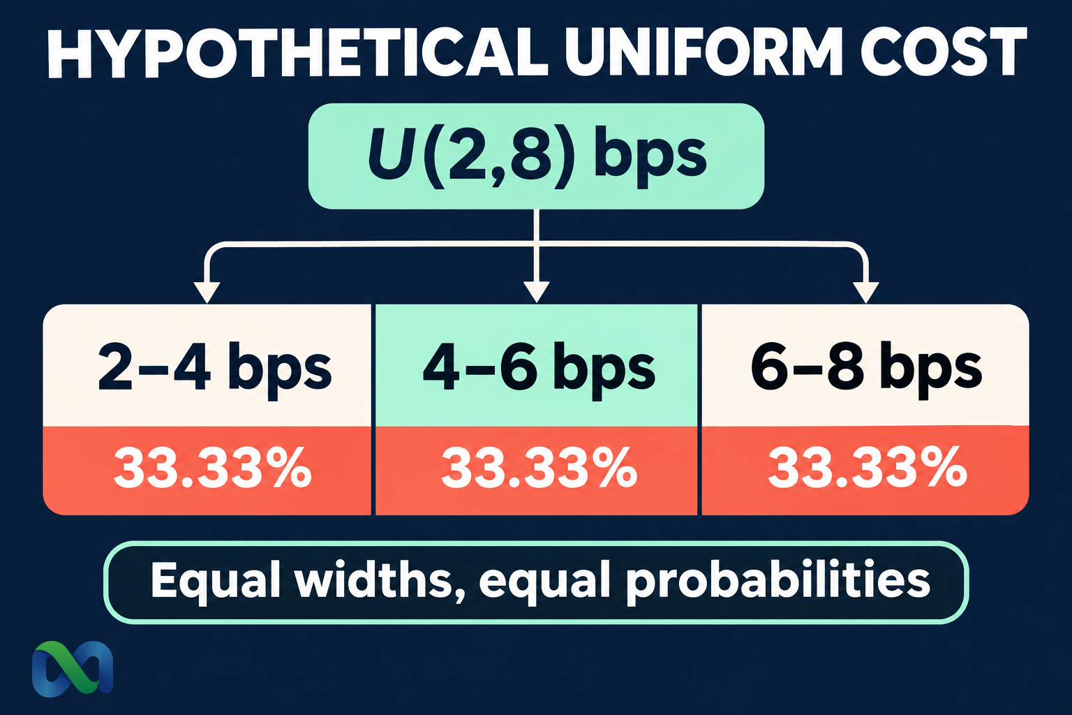
Suppose a simulation models a hypothetical execution cost as uniformly distributed between two and eight basis points. A cost between two and four basis points has the same probability as a cost between six and eight: one-third. The model deliberately treats those equal-width intervals alike; real costs are not automatically uniform.
This guide explains the continuous and discrete formulas, calculates probabilities and summary statistics, and shows how uniform draws are used in simulations. The cost range is an illustrative modeling assumption, not a quote, fee schedule, or observation from Macro Markets.
What Is a Uniform Distribution?
A continuous uniform variable X on the interval from a to b is written X ~ U(a, b), with b > a. Its probability density is flat within that range and zero outside it. The density is 1/(b − a), making the total area under the density equal to one.
NIST’s uniform-distribution reference gives this density and its summary statistics. Equal probability applies to intervals with equal width, not to a positive probability assigned to each individual real number.
For a continuous variable, the probability of any one exact value is zero. That does not prevent an observation from taking a particular value. Probability is obtained by measuring an interval’s area under the density.
A discrete uniform variable is different. If it has m listed possible outcomes, each has probability 1/m. The list matters: seven integer costs from two through eight are a different model from every real-valued cost between two and eight.
Continuous Uniform Distribution Formula
For values inside the support, the probability density function is:
f(x) = 1/(b − a), for a ≤ x ≤ b
For an interval entirely within that support:
P(c ≤ X ≤ d) = (d − c)/(b − a)
The numerator measures the interval’s width. The denominator measures the total support width. If an interval extends outside the support, first restrict it to the overlap with [a, b]. An interval wholly outside has probability zero.
The cumulative distribution function, or CDF, is zero below a, equals (x − a)/(b − a) within the support, and is one above b. It answers the question “What is the probability that X is at most x?”
The model is simple because its only parameters are the lower and upper bounds. That simplicity is useful for a transparent sensitivity assumption. It is also restrictive: a flat density cannot represent a central peak, an asymmetric concentration, or outcomes beyond the bounds.
Worked Example: A Modeled Cost Range
Assume an execution-cost scenario with X ~ U(2, 8), measured in basis points. One basis point is 0.01 percentage point. The support width is six basis points, so the density is 1/6 per basis point.
To calculate the chance of a cost between three and five basis points, divide the interval width by the support width:
P(3 ≤ X ≤ 5) = (5 − 3)/(8 − 2) = 2/6 ≈ 33.33%
The chance of a cost at most six basis points is:
P(X ≤ 6) = (6 − 2)/6 = 4/6 ≈ 66.67%
The three equal-width regions below cover the entire support. Costs and widths in the table are measured in basis points:
| Cost | Width | Probability |
|---|---|---|
| 2–4 | 2 | 33.33% |
| 4–6 | 2 | 33.33% |
| 6–8 | 2 | 33.33% |
The exact probabilities sum to one. The displayed rounded percentages sum to 99.99%, a rounding difference rather than missing probability. Shared interval endpoints cause no double-counting because exact points have zero probability in this continuous model.
Convert the modeled cost into dollars
For a hypothetical $10,000 transaction amount, five basis points corresponds to $5, calculated as $10,000 × 5/10,000. Under the uniform assumption, the modeled cost would range from $2 to $8 on that same amount.
This conversion does not establish an actual charge or include every execution expense. It simply translates a basis-point assumption into currency. Real transaction costs can depend on order size, spread, liquidity, order type, and timing.
Mean, Variance, and Standard Deviation
For a continuous uniform distribution, the mean and median are both (a + b)/2. The variance is (b − a)²/12, and the standard deviation is (b − a)/√12.
With a = 2 and b = 8, the mean is five basis points. The variance is three basis points squared, and the standard deviation is approximately 1.732 basis points. These are population characteristics of the hypothetical model, not estimates calculated from observed trading data.
The mean lies at the midpoint because the density is symmetric. It does not imply that a small interval around five is more probable than an equally wide interval near either endpoint. Every equal-width interior interval has the same probability.
Our variance guide explains why variance has squared units, while standard deviation returns dispersion to the original measurement units. Neither statistic changes the uniform model’s flat density or hard boundaries.
Uniform Distribution Percentiles
The quantile at cumulative probability q is:
xq = a + (b − a)q, for 0 ≤ q ≤ 1
For the hypothetical cost model, the 90th percentile is 2 + 6 × 0.90 = 7.4 basis points. The model assigns 90% probability to costs at or below that threshold and 10% to costs above it.
The 25th and 75th percentiles are 3.5 and 6.5 basis points. The middle 50% therefore occupies a three-basis-point interval. These are distribution percentiles, not confidence limits for an estimated mean.
If the bounds were estimated from a small sample, their uncertainty would need separate attention. Treating the observed minimum and maximum as guaranteed future limits can exclude unseen costs. A bounded model is an assumption about possible values, not a conclusion automatically justified by the current sample range.
Discrete vs. Continuous Uniform Models
Suppose costs could take only the seven integer values 2, 3, 4, 5, 6, 7, and 8, each with equal probability. Each exact cost would then have probability 1/7. A cost of three, four, or five would have combined probability 3/7 ≈ 42.86%.
That differs from the continuous model’s 33.33% probability for the interval from three through five. In the discrete model, three allowed outcomes are counted. In the continuous model, an interval of width two is measured.
The two models share a midpoint of five, but they have different variances. The seven-point discrete example has variance four basis points squared, compared with three for the continuous U(2, 8) model. Matching endpoints and mean does not make the distributions interchangeable.
Choose the model based on how the quantity is defined and recorded. Rounded observations from a continuous process do not necessarily imply a discrete uniform population. Equally spaced allowed values also need not be equally probable.
Uniform Random Numbers in Monte Carlo Simulations
A uniform draw U on [0, 1] can be transformed into a draw on [a, b] using a + (b − a)U. With U = 0.25 in the cost example, the transformed value is 3.5 basis points. With U = 0.75, it is 6.5 basis points.
Uniform numbers can also serve as inputs to transformations that generate nonuniform variables. Using uniform random numbers inside an algorithm does not mean its final simulated costs, returns, or event counts are uniform.
SciPy’s uniform-distribution documentation specifies the lower-bound location and width parameters. For this example, the location is two and the scale is six, not eight. Confusing an upper endpoint with a scale changes the support.
Our Monte Carlo simulation guide explains how assumptions feed simulated outcomes. More simulation runs improve numerical precision within the chosen model; they do not supply evidence that its flat cost density matches actual execution.
Spreadsheet Calculation and Model Checks
In an English-language spreadsheet, =2+(8-2)*RAND() generates a simulated continuous cost using the hypothetical bounds. RAND() produces values from zero up to, but not including, one. Excluding one endpoint does not alter the theoretical continuous probabilities.
For an interior threshold in cell B2, the cumulative probability is =(B2-2)/(8-2). To handle thresholds outside the support, use =MAX(0,MIN(1,(B2-2)/(8-2))). Confirm that the upper bound exceeds the lower bound before dividing.
Random spreadsheet draws recalculate. Save the realized values if another reader must reproduce the same scenario results. A formula screenshot alone may not preserve the draws used for an earlier conclusion.
Compare the model with the question it is meant to answer. Ask why the bounds are plausible, why equal-width intervals should have equal probability, and whether costs can exceed the assumed maximum. If those choices are merely convenient, label the result a sensitivity scenario rather than an empirical forecast.
Frequently Asked Questions
Is a uniform distribution the same as having no information?
No. Selecting a uniform model specifies bounds and a probability structure. A flat density in one measurement scale may become nonuniform after a nonlinear transformation. The choice needs an explanation tied to the variable and modeling purpose.
Can a probability density exceed one?
Yes. Density has inverse measurement units; it is not itself a probability. A uniform variable on an interval of width 0.2 has density five within that interval, while the total area remains one.
Are real market outcomes uniformly distributed?
They are not uniform by default. A uniform distribution can be a useful teaching model, sampling mechanism, or explicit stress-test assumption. Its suitability for an actual variable requires evidence about that variable, its support, and the task.
