


ANOVA Explained: Assumptions, Formula and Worked Examples

ANOVA, short for analysis of variance, is a family of methods for comparing means by examining variation. A one-way ANOVA asks whether several population means can reasonably be treated as equal under a stated model. It separates variation between groups from variation within them.
The method is useful when a report shows different average outcomes for several groups and the next question is whether those differences are large relative to the noise. Different sample averages alone do not show different population means.
What One-Way ANOVA Tests
In a one-way design, one categorical factor identifies the groups. The response is numeric. A hypothetical study might compare a standardized net payoff across three research methods, with independent data points assigned to each method.
The null hypothesis states that all the population means are equal. The alternative is that at least one differs. Rejecting the null does not show that every pair differs, identify the best group or show why any difference exists.
The NIST overview of one-way ANOVA introduces the decomposition of variation. Its ANOVA table and testing explanation connects sums of squares, degrees of freedom and the F statistic. The example below uses a separate small data set to make those calculations reproducible.
Between-Group and Within-Group Variation
First compute each sample's mean and the grand mean of all data points. Between-group variation measures how far the group means lie from the grand mean, accounting for group sizes. Within-group variation measures how far individual data points lie from their own group's mean.
For k groups and N data points, the relevant degrees of freedom are k − 1 between groups and N − k within groups. Divide each sum of squares by its degrees of freedom to obtain a mean square.
F = between-group mean square / within-group mean square
Under the classical model, both mean squares estimate the common error variance when population means are equal. A large ratio can thus provide evidence against equal means. The F reference distribution depends on both degrees of freedom, not on the ratio alone.
Our variance guide explains squared deviations from a mean. ANOVA organizes those deviations into components that answer a comparison question; it is not simply a test of whether the group variances differ.
Worked Example: Three Hypothetical Methods
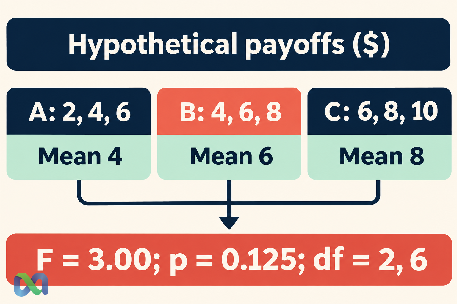
Suppose a teaching exercise records three independent net-payoff data points for each of three methods, with all amounts measured in dollars over the same type of case. Assume equal stakes and a comparable review design. These are hypothetical values, not platform or strategy performance records.
| Method | Observations | Mean |
|---|---|---|
| A | 2, 4, 6 | $4 |
| B | 4, 6, 8 | $6 |
| C | 6, 8, 10 | $8 |
There are nine data points. Their grand mean is $6. The group means differ in the sample, but each group also contains variation around its own mean.
The between-group sum of squares is:
3 × (4 − 6)² + 3 × (6 − 6)² + 3 × (8 − 6)² = 24
Inside each group, deviations from its mean are −2, 0 and 2. Their squared sum is 8, giving a combined within-group sum of squares of 24. The corrected total sum of squares is 24 + 24 = 48.
The degrees of freedom are 3 − 1 = 2 between groups and 9 − 3 = 6 within groups. The mean squares are thus 24 / 2 = 12 and 24 / 6 = 4:
F = 12 / 4 = 3.00
Using an F distribution with 2 and 6 degrees of freedom, the upper-tail p value is 0.125. At a preselected significance level of 0.05, this procedure does not reject equal population means.
The sample means remain $4, $6 and $8. Failure to reject does not erase those descriptive differences or prove that all methods are equivalent. It says the test did not show a population-mean difference under the stated model and decision rule.
Read an ANOVA Table Without Losing the Units
An ANOVA table often compresses several quantities into one display. For the worked example, the sums of squares and mean squares are measured in squared dollars. The F statistic is a ratio of quantities with matching units, so it is dimensionless.
| Component | SS | df |
|---|---|---|
| Between | 24 | 2 |
| Within | 24 | 6 |
| Total | 48 | 8 |
Divide each component's SS by its df before forming the ratio. Comparing the raw sums of squares would give 24 / 24 = 1 and miss the actual F statistic of 3. The degrees-of-freedom adjustment is part of the calculation.
The word “error” in an ANOVA table refers to residual variation under the model. It does not mean someone entered the data incorrectly. Likewise, a group effect in the table describes a statistical component, not by itself a causal influence.
The P Value guide explains how to read a tail probability. In this setting, 0.125 is not a 12.5% probability that the three means are equal.
Check the Assumptions and Design
Classical one-way ANOVA assumes a suitable independent-error model, a common within-group variance and normally distributed errors for its usual exact F inference. The assumptions concern the model and design, not just the appearance of a spreadsheet.
Repeated forecasts on the same event are not independent cases just because they occupy separate rows. If each method is evaluated on the same events, the paired structure may require a repeated-measures or other suitable approach. Random assignment and sampling should be described accurately.
The three data points per group in the example are enough to demonstrate arithmetic, but offer little basis for diagnosing real-world distributions. Do not treat this tiny exercise as a recommended study size or as validation of the normal-error assumption.
Inspect unusual data points and differences in spread. A standard deviation can help summarize within-group variability, while plots and the design provide more context. If equal variance is not defensible, consider a procedure designed for unequal variances rather than selecting whichever result looks more favorable.
Other questions may require another model altogether. Counts, repeated measurements, strongly constrained outcomes and changing exposures should not be forced into a standard one-way calculation solely because the software offers an ANOVA button.
What a Significant Result Would and Would Not Show
If a suitable ANOVA rejects equal means, the next question is which differences matter. The overall test alone does not identify a specific pair. Planned contrasts or suitable multiple-comparison procedures can address those comparisons while accounting for the testing design.
Report the size of the estimated differences and their uncertainty. A small difference can become statistically detectable with a large informative sample, while a financially meaningful difference can remain uncertain in a noisy small sample.
Use confidence intervals to communicate uncertainty when the chosen interval procedure fits the design. State whether an interval concerns a group mean, a difference between means or an individual future data point.
Causation requires more justification. Groups may differ in case difficulty, stake sizes, selection criteria or market conditions. A difference attributed to a method could reflect these other factors if the study does not separate them.
Use ANOVA in Financial Research Carefully
Keep the response variable consistent. Comparing dollar payoffs from positions of very different sizes can mix method performance with exposure. Normalizing a response may help answer one question while creating another; document the choice and its effects.
Evaluation periods also need attention. Overlapping returns or common settlement events can create dependence. Cases collected under different rules may not represent a stable repeated process. A clean calculation cannot compensate for an ill-defined sample.
Separate exploratory analysis from confirmation. Finding groups after searching the outcomes is a different process from testing groups stated in advance. Retain the record of how the factor, filters and comparisons were chosen.
For the hypothetical example, the defensible conclusion is modest: the three sample averages differ, but a classical one-way F test yields 3.00 and p = 0.125 under its assumptions. Future performance and an executable trading advantage remain separate questions.
Frequently Asked Questions
Does ANOVA compare means or variances?
The one-way F test uses variance estimates to assess equality of population means. A direct question about equality of variances requires a suitable variance-comparison procedure.
Does rejection mean every group differs?
No. The alternative says at least one population mean differs. Use justified follow-up comparisons to investigate which differences are supported.
Does a nonsignificant result prove the methods are equivalent?
No. The available sample may leave uncertainty about meaningful differences. Equivalence requires its own question, tolerances and analysis.
Can I compare methods on the same forecast events?
Yes, but the analysis must account for the resulting pairing or repeated measurements. Treating those data points as independent groups can misrepresent uncertainty.
