


Base Rate Fallacy: Meaning and Worked Forecast Examples

The base rate fallacy means giving too little weight to how common an event was before a new signal arrived. A rare event can produce many false alerts, even with a useful signal. To read an alert well, you need to know both how the signal works and the group it comes from. One impressive detection rate is not enough.
A model that spots 80% of stress events does not imply that 80% of its alerts are true. These questions start with different groups. One starts with event cases and asks which were flagged. The other starts with alerts and asks which cases had the event. Mixing those groups can make a forecast look much stronger than it is.
This guide works through a hypothetical financial-stress screen using counts you can check by hand. It shows how the starting rate and false alerts shape the answer, then explains what two signals add when they agree. None of the figures are real default rates, product statistics, or Macro Markets forecasts. The point is to read evidence with the right denominator, not to treat any alert as proof.
What Is a Base Rate?
A base rate is the frequency or prior probability of an event within a defined reference population. The population, event definition, and time horizon all matter. A one-year stress-event rate among a selected group of issuers is not automatically appropriate for a different group or a different horizon.
Let E denote the event and + denote a positive signal. The base rate is P(E). The signal's true-positive rate is P(+ given E), and its false-positive rate is P(+ given not E).
The probability usually wanted after an alert is P(E given +). That is a posterior probability. It combines the base rate with the relative likelihood of seeing the signal when the event occurs and when it does not.
OpenStax's probability-theory chapter presents Bayes' theorem as a way to update a probability when new evidence arrives. The base rate is an input to that update, not information that becomes irrelevant as soon as a signal appears.
The Base Rate Fallacy Formula
For a positive signal, Bayes' theorem gives:
P(E given +) = [P(+ given E) × P(E)] / P(+)
The denominator includes both ways a positive signal can occur:
P(+) = P(+ given E) × P(E) + P(+ given not E) × P(not E)
Leaving out the second term treats false alerts as if they do not exist. Replacing the posterior with the true-positive rate reverses the conditioning. Both mistakes can produce a much stronger-looking forecast than the assumptions support.
The Bayes' theorem guide develops the general update. Here, the emphasis is on choosing a relevant prior population and counting all the alerts in the denominator.
Do not summarize a signal as “80% accurate” unless that term has been defined. Accuracy can refer to several different quantities, and an overall classification accuracy can conceal poor performance on a rare event.
Worked Example: An 80% Detection Rate and a 14% Posterior
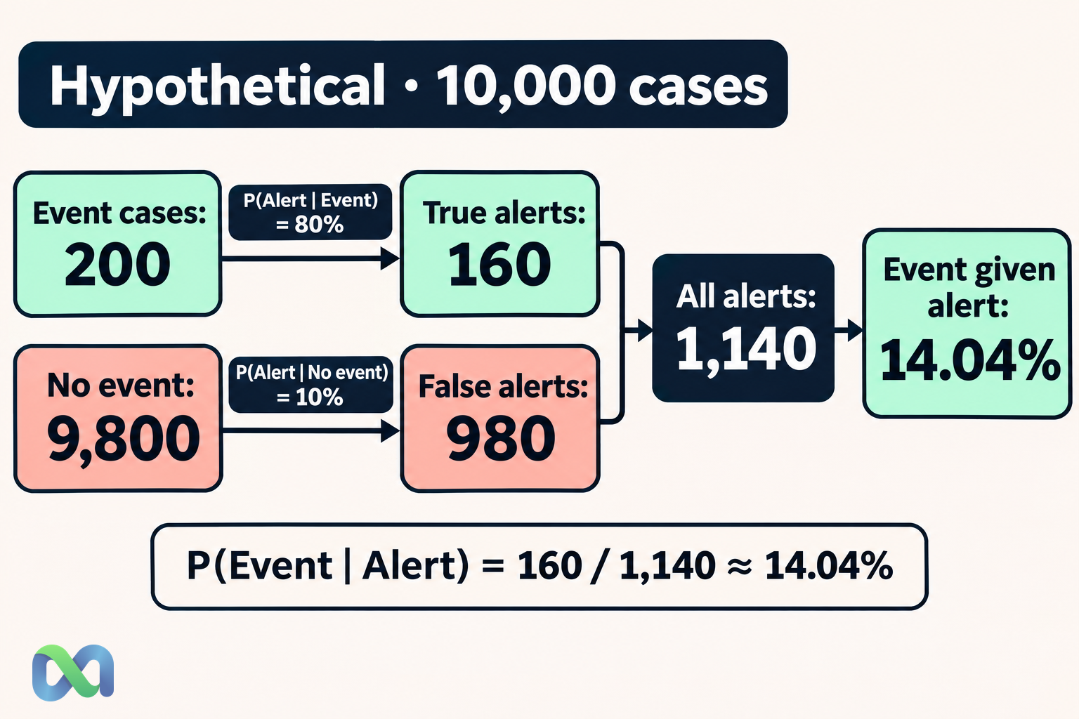
Consider 10,000 hypothetical issuer-year cases. Define E as a specific stress event within one year. Assume its base rate is 2%, the screening process flags 80% of event cases, and it also flags 10% of cases without the event.
There are 200 event cases and 9,800 nonevent cases in this hypothetical population. The signal flags 160 of the event cases and 980 of the nonevent cases. Total positive signals equal 1,140.
| Group | Cases | Alerts |
|---|---|---|
| Event | 200 | 160 |
| No event | 9,800 | 980 |
| Total | 10,000 | 1,140 |
Among the positive signals, the event share is:
160 / 1,140 ≈ 14.04%
The signal raises the event probability from 2% to about 14%. That is a large update, but it remains far below 80%. Most positive signals in this example arise from the much larger nonevent group.
These counts are exact for the constructed population. In a real application, estimated base rates and detection rates would have uncertainty, and the sample used to estimate them might differ from the population being screened.
Change the Base Rate, Keep the Signal the Same
Now keep the true-positive rate at 80% and the false-positive rate at 10%, but change the event's prior probability. The posterior changes even though the assumed signal performance stays fixed.
| Prior event rate | Event chance after + |
|---|---|
| 2% | 14.04% |
| 10% | 47.06% |
| 20% | 66.67% |
At a 20% prior, a hypothetical population of 10,000 cases contains 2,000 event cases and 8,000 nonevent cases. Positive signals then include 1,600 true alerts and 800 false alerts, giving 1,600/2,400 = 66.67%.
This comparison shows why a screening model can have different practical meaning across populations. A risk-enriched group can have a different posterior from a broad screening pool. You cannot transfer the posterior between the groups merely because the signal's name or threshold is unchanged.
It also does not prove that the detection rates really remain stable when the population changes. Holding them fixed is a sensitivity assumption for this example, not an empirical finding. The conditional probability guide explains why the conditioning group must stay explicit.
A Useful Signal Can Still Have Many False Alerts
The hypothetical signal is eight times as likely under E as under not E, because 0.80/0.10 = 8. That likelihood ratio favors the event. The low posterior is therefore not evidence that the signal contains no information.
The starting population, however, contains 49 nonevent cases for every event case. An informative signal has to overcome that imbalance before the event becomes the more common explanation of a positive result.
This observation separates two decisions. One decision concerns how much to update a probability. Another concerns what action, if any, is justified by the updated probability. The costs of false alerts and missed events can make a low-posterior alert worth investigating without making the event more likely than not.
In a financial setting, action also depends on price and payoff. The expected value formula guide shows why the probability alone does not determine whether a position is attractive. An informative forecast is not automatically an economic advantage at every available price.
What Happens When Two Signals Agree?
Two positive signals can provide more evidence, but only after their dependence is considered. Suppose two signals each have the rates used above and are independent conditional on event status. This is a strong extra assumption.
With a 2% prior, the chance of two positives is 0.80^2 = 0.64 for event cases and 0.10^2 = 0.01 for nonevent cases. The posterior after both positives is:
(0.02 × 0.64) / [(0.02 × 0.64) + (0.98 × 0.01)] ≈ 56.64%
You cannot use that calculation merely because two different websites repeat the same alert. They may rely on the same filing, analyst, data feed, or model. Duplicate reporting can add much less information than conditionally independent evidence.
When dependence is unknown, avoid mechanically multiplying likelihoods. Trace each signal to its underlying information and test whether the model accounts for the overlap. The independent events guide introduces independence; conditional independence is the more specific requirement used in this two-signal example.
Reproduce the Posterior in a Spreadsheet
Put the prior event probability in B2, true-positive rate in B3, and false-positive rate in B4. With the example inputs 0.02, 0.80, and 0.10, use:
=(B2*B3)/(B2*B3+(1-B2)*B4)
The result is about 0.140350877, which displays as 14.04% when rounded to two decimal places. Check that the denominator is positive; if the model assigns zero probability to any positive signal, conditioning on a positive signal is undefined within that model.
For a natural-frequency check with 10,000 hypothetical cases, calculate event cases as =10000*B2, true alerts as =10000*B2*B3, and false alerts as =10000*(1-B2)*B4. Divide true alerts by total alerts. The formula and the frequency calculation should agree.
Keep the rate definitions visible beside the cells. A correct formula applied to a precision estimate where a true-positive rate was required still answers the wrong question.
How to Avoid the Base Rate Fallacy in Forecasting
Choose the reference class before selecting a convenient probability. Define the event, population, and horizon, then explain why that class is relevant to the new case. Very broad classes can ignore meaningful differences; very narrow classes can leave too little evidence to estimate reliably.
Separate the prior, the new evidence, and the update. This makes it easier to see whether an analyst has counted the same information twice. If the prior already incorporates a public filing, treating that filing as a fresh independent signal can overstate the update.
Audit performance on data that were not used to choose the signal threshold. Retain false alerts and missed cases, and check whether the relevant rates change over time. More decimal places cannot repair selection bias or an outdated reference population.
Frequently Asked Questions
Is the base rate fallacy the same as ignoring all new evidence?
No. It usually involves underweighting the prior frequency relative to new evidence. The goal is to combine both appropriately, rather than always favoring the prior or always favoring the signal.
Does a low posterior mean the signal is useless?
No. In the example, the signal increases probability from 2% to about 14%. Whether that update warrants an action depends on the consequences and costs of the available actions.
Can I use a historical average as the base rate?
Only after checking whether its event definition, population, horizon, and conditions are relevant. A historical average is an estimate with limitations, not a universal prior for every new case.
Should two agreeing forecasts count as two signals?
Only to the extent that they contribute distinct information under a defensible model. Shared sources and copied reasoning can make apparently separate forecasts highly dependent.
