


Central Limit Theorem: Meaning, Examples and Financial Limits

The central limit theorem explains why averages can have an approximately normal sampling distribution even when individual observations are not normally distributed. The theorem concerns the behavior of a properly standardized sum or mean as sample size grows. It does not make every large dataset normal.
Consider a hypothetical waiting time with an exponential distribution, a mean of five minutes, and a standard deviation of five minutes. An individual wait is right-skewed. An average of 100 independent waits is much less variable, with a standard deviation of 0.5 minutes, and its sampling distribution can be approximated by a normal distribution.
This distinction matters when reading financial averages, simulated outcomes, and estimates of event frequencies. The examples below separate the underlying observations from the distribution of their averages and explain why dependence and heavy tails require extra care.
What Does the Central Limit Theorem Say?
In its classical independent and identically distributed form, the central limit theorem assumes observations with a common finite mean μ and a common finite, positive variance σ². As n increases, the standardized sample mean converges in distribution to a standard normal random variable.
The standardized expression is:
Zₙ = (X̄ − μ) ÷ (σ/√n)
For a sufficiently large sample under those conditions, it is approximately distributed as N(0, 1). Equivalently, the sample mean is approximately normal with mean μ and variance σ²/n. The denominator σ/√n is the standard deviation of the sample mean.
OpenStax’s sampling-distribution lesson develops the relationship between the population, sample means, and their standard errors. The approximation concerns repeated samples of the same size from the same process. One observed average is a single value from that conceptual sampling distribution.
Other central limit theorems relax the identical-distribution or independence conditions, but they introduce their own requirements. You cannot assume that a dependent financial series satisfies one merely because the classical version is familiar.
Individual Observations vs. Sample Means
Imagine three separate objects: a population distribution of waiting times, one sample of 100 waits, and a distribution of averages obtained by repeating that 100-observation sample many times. The central limit theorem addresses the third object.
Adding more waits to a histogram of individual exponential observations reveals the right-skewed population shape more clearly. It does not turn that histogram into a bell curve. Taking the mean within each new sample, however, creates a different random variable with different dispersion.
This is why “we have thousands of returns, so returns are normal” is a faulty argument. A large number of return observations does not change their underlying distribution. Even an approximate normal model for an average does not automatically produce an accurate model for an extreme individual loss.
The normal distribution guide explains the properties of a normal variable. NIST’s normal-distribution reference provides the density and parameter definitions. Those properties apply when a normal model is justified; sample size alone does not justify every application.
Worked Example: Average Waiting Time
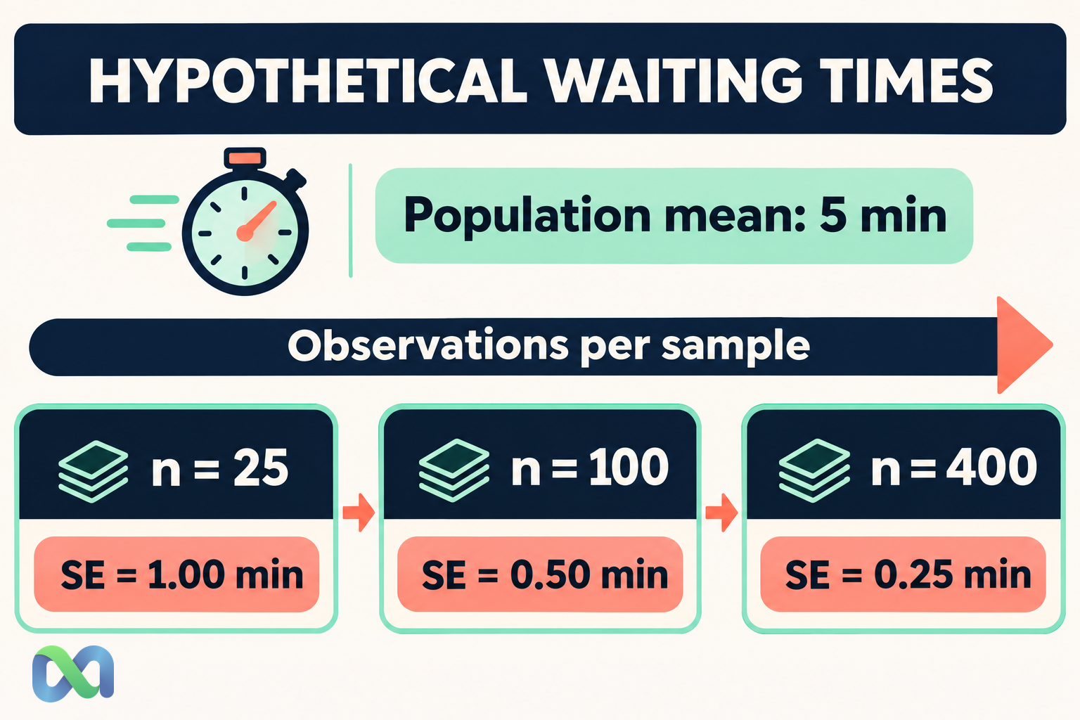
Assume independent waiting times from an exponential population with mean μ = five minutes and standard deviation σ = five minutes. Every observation is nonnegative, and the population is right-skewed. The values are hypothetical and describe no particular trading venue or service.
The mean of n observations has expected value five minutes. Independence gives it variance 25/n minutes² and standard deviation 5/√n minutes. These moment relationships are exact for this model; normality of the sampling distribution is an approximation.
| n | Mean (min) | SE (min) |
|---|---|---|
| 25 | 5 | 1.00 |
| 100 | 5 | 0.50 |
| 400 | 5 | 0.25 |
At n = 100, an approximate central 95% sampling band is:
5 ± 1.96 × 0.50 = 4.02 to 5.98 minutes
This calculation assumes that the population mean and standard deviation are known model inputs. It describes where averages from repeated samples would tend to fall. It is not a confidence interval estimated from a particular observed dataset.
Notice what changes when n rises from 25 to 100. The standard error halves, although sample size quadruples. The expected average remains five minutes. More observations tighten the distribution of the average without changing the population’s expected waiting time.
The Theorem in a Binary-Event Example
Let each of 100 hypothetical independent events have probability p = 0.60. Set Xᵢ = 1 if event i occurs and zero otherwise. Each individual variable is Bernoulli, so it takes only two values rather than forming a continuous bell curve.
The average X̄ is the fraction of events that occur. Its mean is 0.60, and its standard error is:
√[p(1 − p)/n] = √(0.60 × 0.40/100) ≈ 0.0490
That is about 4.90 percentage points. For 400 comparable independent events, the standard error would be about 2.45 percentage points. These calculations assume a common probability that is known for the example; they do not estimate forecast uncertainty for an actual event.
The binomial distribution provides the exact count probabilities. A normal approximation can be useful when the count has sufficient mass away from both endpoints, but the discrete support remains. For a probability near zero and a modest n, the approximation may perform poorly even if n exceeds a familiar classroom threshold.
Is a Sample Size of 30 Enough?
There is no universal sample size that guarantees an accurate normal approximation for every population and every question. The required n depends on skewness, tail behavior, the precision needed, and whether you care about the center or an extreme tail.
If observations are already independent and normally distributed, their average is normal for any positive n. A strongly skewed distribution can need more observations for a useful approximation. A heavy-tailed distribution can converge slowly. A population without a finite variance falls outside the classical theorem stated here.
Even within the classical conditions, an approximation that is acceptable near the center can be inadequate for a very small tail probability. A risk assessment concerned with rare losses should test the relevant tail, rather than rely on a bell-shaped plot of average outcomes.
Choose the approximation after inspecting the model and the task. Where an exact distribution is available, compare it. Where simulation is appropriate, verify the model inputs and measure the approximation error at the thresholds you will use.
Central Limit Theorem vs. Law of Large Numbers
The law of large numbers and the central limit theorem describe related but distinct behavior. The law of large numbers concerns the tendency of the sample average to approach the population expectation under suitable conditions. The central limit theorem describes the limiting distribution of the standardized error around that expectation.
For the hypothetical waiting-time model, both point to a more stable average as n grows. The law of large numbers supplies the convergence idea. The central limit theorem supplies an approximate shape and the square-root scaling used to assess fluctuations of the mean.
Neither theorem says that an average must move closer to its target after every additional observation. A new observation can move it farther away. Neither says that a sequence of losses makes a compensating win due.
Our law of large numbers explanation develops that distinction. When discussing a sample, identify whether the claim concerns convergence, the shape of sampling error, or the distribution of individual outcomes. Naming the relevant object prevents many common errors.
Why Financial Dependence Changes the Calculation
For independent observations with common variance σ², the variance of their mean is σ²/n. With dependent observations, covariance terms also enter. Positive covariance can make the mean much more variable than the independence formula suggests.
One hundred positions exposed to the same announcement are not equivalent to one hundred independent experiments. Daily returns with serial dependence and overlapping holding periods also need a model that reflects those relationships. More rows can provide less additional information than their count suggests.
A changing process creates another problem. Combining observations from different trading rules, cost structures, or market regimes may not represent repeated sampling from a single stable population. A normal approximation cannot resolve an unclear target.
This affects Monte Carlo simulations too. Independent simulation draws from a specified model can allow a precise estimate of that model’s expected output. They do not prove that the model captures real dependence, rare events, or structural changes. Simulation error and model error are separate questions.
How to Check a Practical Application
Start by defining the random variable and the unit of observation. State whether you are studying one result, a sum, a sample mean, or an estimated proportion. Then document the assumptions that justify the sampling distribution.
Check how observations are related. If they share an event, source, time window, or exposure, do not assume independence. Inspect the distribution for extreme values and consider whether a finite-variance model is credible for the intended calculation.
For a reproducible teaching simulation, repeatedly draw n values from a specified distribution, calculate one mean per sample, and examine those means. Keep the number of observations per sample separate from the number of repeated samples. Increasing those two quantities answers different questions.
Finally, compare the approximation against exact calculations or a validated simulation where feasible. Report the sample size and the part of the distribution being assessed. A visual resemblance to a normal curve is useful context, not a guarantee about all probabilities.
Frequently Asked Questions
Does the central limit theorem require a normal population?
The classical theorem does not require normal individual observations. It requires the conditions stated above, including independence, a common distribution, and finite positive variance. A normal population is a special case in which averages are already exactly normal.
Does it apply to prices or returns automatically?
No. You must define the quantity being averaged and assess its dependence, stability, and tail properties. The theorem does not establish that prices, individual returns, or portfolio losses follow a normal distribution.
Does a larger sample remove uncertainty?
Under the model, it reduces sampling variation in the average. It does not eliminate selection bias, measurement errors, dependence, or uncertainty about whether the model represents the population. Those issues need their own checks.
