


Coefficient of Variation: Formula and Financial Examples
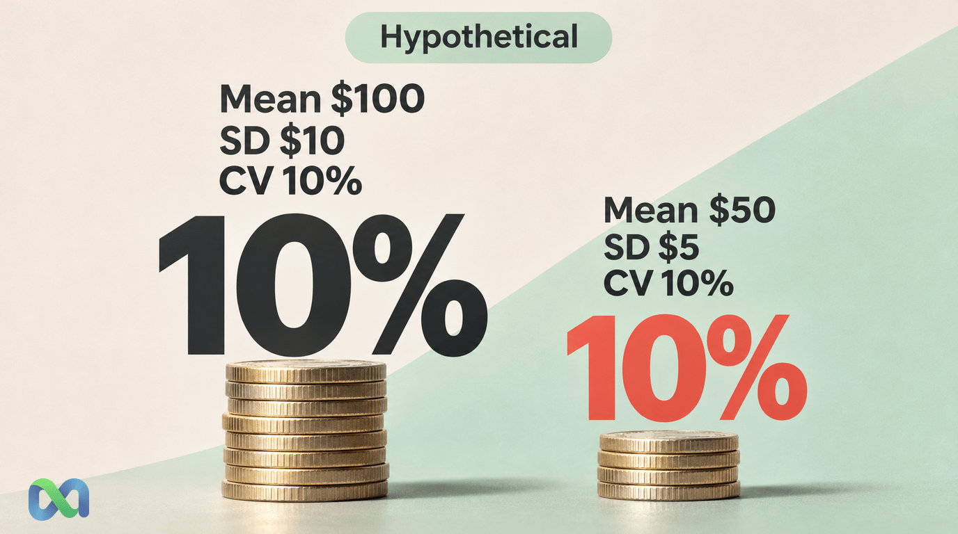
The coefficient of variation, or CV, measures standard deviation relative to the mean. For a sample with a suitable positive mean, divide the sample standard deviation by that mean. Multiply by 100 to express the result as a percentage.
The calculation can help compare relative spread when financial quantities have different scales. It also has important limits: the measurements need a meaningful zero, the mean must be suitable for the comparison, and a small denominator can make the ratio unstable.
The Coefficient of Variation Formula
For sample standard deviation s and sample mean x-bar:
CV = s / mean
CV in percent = 100 × s / mean
For a population description, use the population standard deviation and population mean instead. Identify which version you compute. A sample and population standard deviation use different denominators when computed from the same finite list.
The NIST coefficient-of-variation reference defines the sample ratio and explains its scale and near-zero-mean limitations. Its discussion of scale measures places standard deviation among several ways of describing dispersion.
A CV of 10% means the standard deviation is one-tenth of the mean in that calculation. It does not mean each data point lies within 10% of the mean, that the chance of a loss is 10% or that the figure summarizes every risk in the data.
Worked Example: Payment Amounts on Different Scales
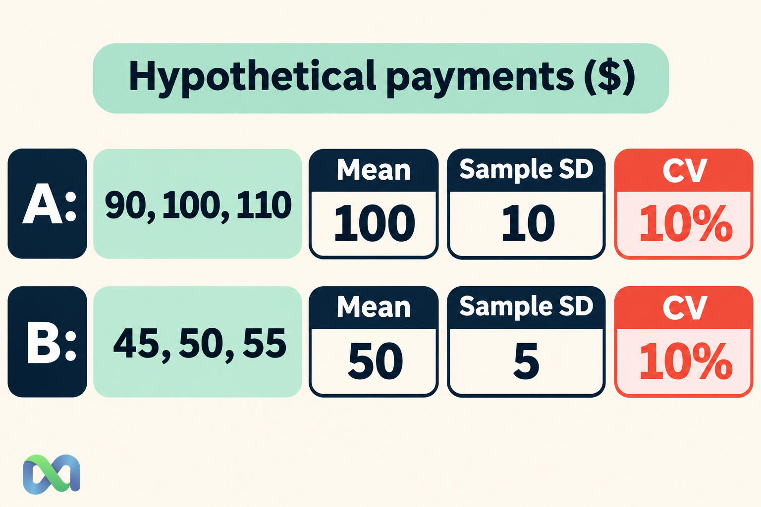
Consider two small hypothetical samples of cash payments, measured in dollars. Sample A contains 90, 100 and 110. Sample B contains 45, 50 and 55. These are illustrative amounts with a meaningful zero, not actual platform transactions.
For sample A, the mean is $100. Deviations from the mean are −10, 0 and 10. Their squared sum is 200. Divide by n − 1 = 2 to obtain sample variance of 100, then take the square root to obtain sample standard deviation of $10.
For sample B, the mean is $50 and the sample standard deviation is $5. The absolute spread is smaller, but so is the mean:
CV(A) = $10 / $100 = 0.10 = 10%
CV(B) = $5 / $50 = 0.10 = 10%
| Sample | Mean / sample SD | CV |
|---|---|---|
| A | $100 / $10 | 10% |
| B | $50 / $5 | 10% |
| C | $100 / $20 | 20% |
The third row uses sample C with payment amounts 80, 100 and 120. It has the same mean as A and twice its sample standard deviation, giving a CV of 20%.
The comparison answers a relative-spread question. It does not rank the payments as investments or show that one collection process is better. With only three data points in each sample, it also does not show stable population differences.
Our standard-deviation guide explains the absolute spread calculation. The variance guide explains the squared deviations and why the sample denominator differs from the population denominator.
Unit Conversion Preserves CV; Adding a Constant Does Not
Convert sample A from dollars into cents. The mean becomes 10,000 cents and the sample standard deviation becomes 1,000 cents. Their ratio remains 1,000 / 10,000 = 0.10.
Multiplying every data point by the same positive constant multiplies the mean and standard deviation by that constant. The constant cancels from the ratio. This is the useful unit-invariance property of CV for a suitable measurement scale.
Now add $900 to every original A data point instead. The new values are $990, $1,000 and $1,010. Their mean is $1,000 and their sample standard deviation remains $10. The CV is now 1%.
That is not a unit conversion. Adding a constant changes the origin or the actual measured amounts. The different ratio shows why the meaning of zero matters to a relative-spread measure.
A ratio-scale quantity has a meaningful zero and supports meaningful multiplicative comparisons. Cash payment amounts can meet that description for a clearly defined payment population. An arbitrary index level or a temperature scale with a conventional zero may not support the same interpretation.
What Happens Near a Zero Mean?
The denominator can dominate the result. As the mean approaches zero while standard deviation remains large, the numeric quotient can become very large. At an exactly zero mean, the formula is undefined.
For example, the signed values −10, 0 and 10 have mean zero. Dividing their standard deviation by that mean cannot produce a valid finite CV. Reporting zero would hide the failure rather than solve it.
Signed return data illustrate another trap. If a return series has a mean of 0.1% and standard deviation of 2%, the numeric ratio is 20, or 2,000%. That arithmetic is correct, but it does not make CV a suitable general-purpose risk measure for signed returns.
A slightly different estimated mean can change that quotient sharply, including its sign. Replacing the mean with its absolute value changes the statistic; it should not be done silently to obtain a more attractive or interpretable result.
Before using the ratio, inspect the underlying mean and standard deviation separately. An extreme CV can show a problematic denominator or measurement scale rather than a newly discovered level of economic risk.
CV Is Not the Sharpe Ratio
CV compares standard deviation with the raw mean of a suitable variable. A conventional Sharpe ratio compares mean excess return with return volatility, using a stated risk-free benchmark and consistent measurement period.
Even where both can be computed numerically from a return sample, they answer different questions. The presence of a benchmark, the direction of the ratio and the treatment of signed returns all matter. Do not describe a low CV as a guaranteed improvement in risk-adjusted investment performance.
The Sharpe ratio guide explains that separate framework and its assumptions. Neither ratio captures every feature of a distribution, such as liquidity constraints, extreme losses or changing exposure.
CV also does not measure forecast calibration. A narrow spread of probability estimates might show a stable forecasting process, or just a process that rarely changes its mind. Accuracy and calibration require outcomes and a suitable review design.
Skewed Data and Uncertainty Still Matter
Two samples with similar CVs can have different shapes and tail behavior. Looking only at the ratio can hide a few very large data points or a multimodal pattern. Inspect the distribution and retain the absolute units alongside the relative summary.
For positive skewed quantities, a lognormal distribution may be relevant in some models. That is a modeling decision, not a reason to label every positive cash amount lognormal. Check the process and data before adopting a distributional formula.
A sample CV is itself an estimate. Its precision depends on the sampling design, sample size and distribution. The five digits a spreadsheet can display do not create five digits of reliable information.
If the goal is an interval estimate or a comparison across populations, use a method suitable for that question and its assumptions. Calculating s / mean alone does not provide a confidence interval or prove a difference between two underlying populations.
A Practical Calculation Routine
Define what each data point represents and the common time period. Separate payment amounts from return percentages, levels from changes and a numeric index from a quantity with a meaningful zero.
Compute the mean and the chosen standard deviation first. Check missing values, repeated records, weights and unusual data points. If the population being described is unclear, a more precise CV calculation will not repair the interpretation.
Then inspect the denominator. If it is zero, near zero or negative, reassess whether the ratio answers the intended question. Report any limitation directly instead of deleting data points until the quotient looks convenient.
Finally, present the mean, standard deviation, CV, units and sample size together. In the worked example, “mean $100, sample SD $10, CV 10%, n = 3” allows a reader to see exactly what is being summarized. Preserve the distinction between this descriptive calculation and a future financial decision.
Frequently Asked Questions
Is a lower CV always better?
No. It shows less standard deviation relative to the mean for the stated calculation. Whether that is desirable depends on the quantity, objective, measurement scale and other features of the distribution.
Should I use sample or population standard deviation?
Use the version that matches the descriptive or inferential question and label it. The worked example uses sample standard deviation with denominator n − 1.
Can I calculate CV for a zero mean?
No finite ratio is defined by s / mean when the mean is zero. Investigate the scale and choose a suitable alternative description rather than reporting an arbitrary replacement.
Does a CV of 10% mean losses cannot exceed 10%?
No. CV is a relative-dispersion summary, not a bound on outcomes or a probability of loss. Its meaning depends on the variable and does not show a trading guarantee.
