


Lognormal Distribution: Formula and Financial Examples

A lognormal distribution describes a positive variable whose natural logarithm follows a normal distribution. The original variable is right-skewed, while its logarithm is symmetric under the model. Prices and their logarithms therefore have different distributions and different parameter interpretations.
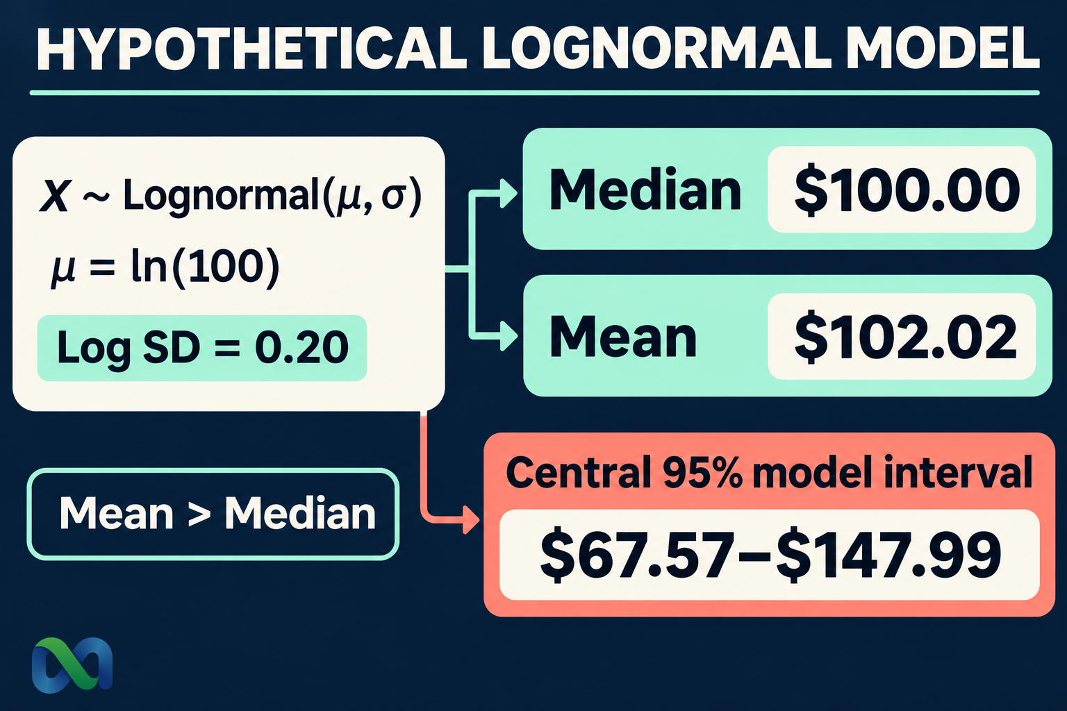
Consider a hypothetical positive value with a modeled median of $100 and a log-scale standard deviation of 0.20. Its mean is approximately $102.02, and its central 95% model interval is approximately $67.57 to $147.99. The interval is asymmetric in dollars because equal movements on the logarithmic scale become multiplicative movements on the original scale.
This guide explains the formulas, works through the example, and distinguishes a lognormal price model from normal log returns. It also explains why an ordinary lognormal model is unsuitable for a probability restricted to zero through one.
What Is a Lognormal Distribution?
For the unshifted two-parameter model used here, ln(X) ~ N(μ, σ²) with σ > 0 and X > 0. Equivalently, X = exp(Y) where Y is normal. The parameters μ and σ describe the logarithm, not the mean and standard deviation of X itself.
NIST’s lognormal-distribution reference defines this relationship and discusses alternative parameterizations. The distinction is essential: setting μ = 100 does not create a lognormal variable with a typical value of $100.
The distribution has a lower bound of zero without positive probability at zero and has no finite upper bound. Its right tail can move the arithmetic mean above the median. A larger log-scale standard deviation increases that separation.
If observations include zero, negative values, or a strict upper limit, this basic model needs reconsideration. Adding a constant or shifting the distribution changes the model and parameter interpretation; it should not be an undocumented fix to force a fit.
Lognormal Distribution Formula
The probability density function is:
f(x) = exp[−(ln(x) − μ)²/(2σ²)] ÷ [xσ√(2π)], for x > 0
The cumulative probability is:
P(X ≤ x) = Φ[(ln(x) − μ)/σ]
Here, Φ is the standard normal cumulative distribution function. To obtain an upper-tail probability, subtract that cumulative probability from one. To obtain the probability between two positive thresholds, subtract their cumulative probabilities.
The units and measurement scale matter. In the example, x is the numerical value measured in dollars, and μ is calculated using that same convention. Changing the currency or numerical unit changes μ and the scale of X; it does not change σ when the conversion is a fixed positive multiplier.
The normal distribution guide explains the normal variable used after taking logs. A normal logarithm does not mean the original dollar value has a normal distribution or symmetric dollar risks.
Mean, Median, Mode, and Variance
For the unshifted model, the median is e^μ, the mean is e^(μ + σ²/2), and the mode is e^(μ − σ²). These represent different features of the same distribution.
The variance is:
Var(X) = (e^(σ²) − 1)e^(2μ + σ²)
The standard deviation is the square root of that expression. It is measured on the original scale, unlike σ, which describes the log scale. The standard deviation guide explains why that unit distinction matters.
For a right-skewed lognormal variable, the mode is below the median, which is below the mean. A single “average” without specifying which measure can therefore obscure a meaningful difference.
The median marks the 50th percentile; the mean summarizes expected magnitude across repeated draws. Neither is guaranteed to occur in one realization, and neither describes uncertainty about a parameter estimated from data. A distribution characteristic and an estimation interval are separate objects.
Worked Example: A $100 Median
Assume μ = ln(100) and σ = 0.20. These are hypothetical inputs for one specified horizon. The example makes no claim about any actual stock, crypto asset, or prediction-market contract.
The median is e^ln(100) = $100. The mean is:
100 × e^(0.20²/2) = 100 × e^0.02 ≈ $102.02
The mode is 100 × e^(−0.04) ≈ $96.08. Applying the variance formula gives approximately 424.76 dollars squared, with a standard deviation of approximately $20.61.
| Measure | Value |
|---|---|
| Mode | $96.08 |
| Median | $100.00 |
| Mean | $102.02 |
| Standard deviation | $20.61 |
These values come from the complete specified distribution. They are not sample statistics and carry no implication that an asset is currently priced at $100 or expected to earn a particular return.
Probability of exceeding $120
Standardize the log threshold:
z = [ln(120) − ln(100)]/0.20 = ln(1.20)/0.20 ≈ 0.9116
The model probability of X ≤ $120 is approximately 81.90%, leaving approximately 18.10% above $120. The calculation answers a threshold question within the hypothetical model. It does not validate the parameter inputs or an asset forecast.
Lognormal Percentiles and Model Intervals
The quantile at cumulative probability q is:
xq = exp(μ + σzq)
Here, zq is the corresponding standard normal quantile. A central 95% interval uses approximately −1.9600 and +1.9600 on the log scale.
For the example, the endpoints are:
Lower = 100 × e^(−1.959964 × 0.20) ≈ $67.57
Upper = 100 × e^(1.959964 × 0.20) ≈ $147.99
The distances from the $100 median differ in dollars. On a multiplicative scale, however, the endpoints use reciprocal factors around the median. Taking logs turns them into equal distances around μ.
This is a central interval for future draws under known model inputs, not a 95% confidence interval for the mean. Parameter-estimation uncertainty is not included. Calling every 95% range a confidence interval blurs what the calculation actually measures.
Normal Log Returns vs. Lognormal Prices
Let a starting positive price be S0 and a later price be ST. The log return is R = ln(ST/S0). If R is normal with mean m and variance v for the specified horizon, then ST = S0 × e^R is lognormal under that model.
The median terminal price is S0 × e^m, while the mean is S0 × e^(m + v/2). The additional v/2 term appears because exponentiation is nonlinear. Exponentiating an expected log return does not generally give the expected terminal price.
This relationship is a model specification, not evidence that actual returns are normal. Jumps, changing volatility, dependence, and extreme events can make a simple normal-log-return model inadequate. The model’s parameters also depend on the time horizon.
Do not turn an assumed log-return standard deviation into an annualized figure without checking the scaling assumptions. The horizon, dependence structure, and meaning of drift all matter. A mathematical transformation can be exact conditional on a model while the model itself remains an imperfect description of markets.
Why Bounded Probabilities Need a Different Model
An ordinary lognormal variable can exceed one by an arbitrarily large amount. A probability must remain between zero and one. Thus directly modeling an event probability or a normalized $1 binary-contract price as unshifted lognormal assigns positive probability to impossible values.
That is a support mismatch, even if many simulated values happen to lie inside the valid range. Clipping the results at one changes the distribution and can create an artificial mass at the boundary. It is not the original lognormal model anymore.
Depending on the question, a bounded model or a transformation such as a logistic function may be appropriate. Choosing one requires specifying whether you are modeling a price, a probability estimate, or uncertainty about an underlying latent variable.
For binary contracts, the expected value formula connects a probability, entry price, and payout. A positive-valued distribution alone does not supply a valid event probability or account for contract fees and settlement terms.
Calculate the Example in a Spreadsheet or Library
In an English-language spreadsheet, =LOGNORM.DIST(120,LN(100),0.2,TRUE) calculates the cumulative probability at $120. Subtract the result from one for the upper tail. =LOGNORM.INV(0.975,LN(100),0.2) gives the upper endpoint of the central 95% interval.
SciPy’s lognormal documentation uses a shape parameter s and a scale parameter. For this example, use s = 0.20, scale = 100, and location = zero. The scale equals e^μ, not μ itself.
Before fitting observations, inspect whether every value is positive and whether the log-transformed data plausibly match a normal model for the intended task. A fit near the center does not establish accurate tail probabilities.
If using the model in a Monte Carlo simulation, record the parameterization, units, horizon, and reason for choosing it. Increasing simulation runs can reduce numerical error while leaving misspecified tails or structural risks unchanged.
Frequently Asked Questions
Is the lognormal distribution the same as the normal distribution?
No. Under a lognormal model, the logarithm is normal. The original variable is positive and right-skewed. A normal variable itself can take negative values and is symmetric about its mean.
Is the log-scale mean the average price?
No. μ is the mean of ln(X) under the chosen measurement convention. The arithmetic mean of X is e^(μ + σ²/2). Confusing the two can substantially change a forecast or simulation.
Can a lognormal model predict prices reliably?
The model produces probabilities conditional on its assumptions and inputs. Its accuracy for an actual asset and horizon must be assessed with relevant data and diagnostics. Positivity and a familiar curve do not by themselves establish predictive accuracy.
