


Covariance: Formula, Examples and Portfolio Risk

Covariance measures how two variables vary together around their respective means. Positive covariance indicates that their deviations tend to have the same sign. Negative covariance indicates that the deviations tend to have opposite signs. Its size depends on the variables’ measurement units.
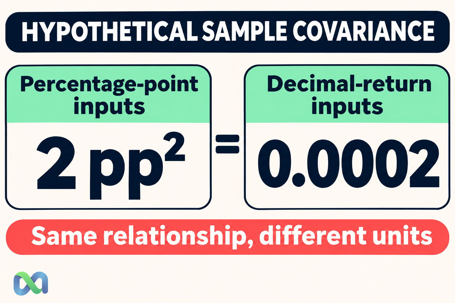
In a hypothetical four-period return example, two assets have a sample covariance of 2 percentage points squared. That same covariance is 0.0002 when both return series are entered as decimals. The economic relationship has not changed; the numerical scale has.
This guide calculates covariance from paired observations, converts it to correlation, and uses it in a two-asset portfolio variance calculation. The short dataset is for arithmetic demonstration, not an estimate of any actual asset’s future relationship or risk.
What Does Covariance Tell You?
Covariance looks at products of deviations from two means. When both variables are above their means, their deviation product is positive. The product is also positive when both are below their means. Opposite-sign deviations produce a negative product.
A positive average of those products indicates co-movement around the respective means. It does not mean that both variables are always positive or that both always rise in every period. It also does not establish that one variable causes the other.
Because covariance retains the variables’ units, its magnitude is not directly comparable across arbitrary measurement scales. A covariance between two returns has different units from a covariance between a price and a trading volume.
For a standardized measure, use the correlation coefficient. Correlation divides covariance by the product of the standard deviations, provided both are positive. Covariance remains useful because its units and cross terms fit directly into portfolio variance calculations.
Population and Sample Covariance Formulas
For random variables X and Y, population covariance is:
Cov(X, Y) = E[(X − μX)(Y − μY)]
An equivalent expression is E[XY] − E[X]E[Y], assuming the required expectations exist. The formula centers each variable before measuring how they move together.
For n paired sample observations, a common sample estimator is:
sXY = Σ[(xi − x̄)(yi − ȳ)] ÷ (n − 1)
Use each xi with the corresponding yi from the same observation period. The n − 1 denominator is the standard sample convention when estimating covariance from independent paired observations with finite second moments.
If the data represent the complete finite population being described, the descriptive population calculation divides by n instead. NumPy’s covariance documentation explains the normalization options and the covariance matrix. Software settings must match the convention you intend to report.
Worked Example: Four Paired Returns
Consider the following hypothetical same-period returns. Numbers are shown as percentages, with deviations calculated in percentage points.
| Period | A | B |
|---|---|---|
| 1 | −2% | −1% |
| 2 | −1% | 0% |
| 3 | 1% | 2% |
| 4 | 2% | 1% |
Asset A has a mean return of zero. Asset B has a mean return of 0.5%. The centered values for A are therefore −2, −1, 1, and 2 percentage points. For B, they are −1.5, −0.5, 1.5, and 0.5 percentage points.
Multiply the paired deviations: the four products are 3, 0.5, 1.5, and 1 percentage points squared. Their sum is six. With four observations, the sample denominator is three:
Sample covariance = 6 ÷ (4 − 1) = 2 percentage points squared
If these four periods were instead treated as the complete population of interest, the descriptive population covariance would be 6/4 = 1.5 percentage points squared. The denominator is the reason for the difference, not a change in the underlying paired data.
This example is intentionally small enough to check by hand. Four periods are not sufficient grounds for a reliable claim about a stable long-run financial relationship. A sample covariance can be calculated precisely while remaining a highly uncertain estimate.
Why Units Change the Number
Entering a 1% return as 0.01 expresses it in decimal units. Entering it as 1 expresses it in percentage-point units. Multiplying every observation of both variables by 0.01 multiplies their covariance by 0.01².
Thus the worked sample covariance becomes:
2 × 0.01² = 0.0002 in decimal-return units squared
Neither result is more positive than the other. They describe the same paired relationship using different units. The conversion matters when combining covariance with variances or checking a spreadsheet against a programming library.
More generally, multiplying X by a constant a and Y by a constant b multiplies covariance by ab. Adding a fixed constant to either variable does not change covariance because centering removes it. Multiplying one variable by a negative constant reverses the sign.
Our variance explanation covers the same squared-unit issue for a single variable. Variance is covariance of a variable with itself. Keeping both measures on a consistent scale prevents silent portfolio-calculation errors.
Covariance vs. Correlation
The sample correlation is:
rXY = sXY ÷ (sX × sY)
In the example, A’s sample variance is 10/3 and B’s is 5/3, both in percentage points squared. Their sample standard deviations are approximately 1.826 and 1.291 percentage points.
The correlation is therefore:
2 ÷ √[(10/3) × (5/3)] ≈ 0.8485
Changing both return series to decimals leaves this correlation unchanged because the scaling cancels between numerator and denominator. Correlation is dimensionless and lies between −1 and 1 when defined. Covariance has no universal numerical range across different units and variances.
A positive correlation of about 0.85 summarizes a strong positive linear relationship in this small sample. It does not guarantee future diversification behavior or rule out joint losses. It also does not say that 85% of one asset’s movements are caused by the other.
Use the standard deviation guide when checking the denominator. If either variable has zero standard deviation, ordinary correlation is undefined; dividing by zero is not a meaningful estimate of a relationship.
Using Covariance in Portfolio Risk
For a two-asset portfolio with fixed weights wA and wB over the measured period, the return variance is:
Var(Rp) = wA²Var(A) + wB²Var(B) + 2wAwB Cov(A, B)
For a 50/50 combination of the hypothetical return series, substitute the sample measures consistently:
Portfolio variance = 0.25 × (10/3) + 0.25 × (5/3) + 0.50 × 2 = 2.25
The units are percentage points squared. The sample portfolio standard deviation is √2.25 = 1.50 percentage points.
You can verify this directly. The portfolio returns for the four periods are −1.5%, −0.5%, 1.5%, and 1.5%. Their mean is 0.25%, and their sample variance is 2.25 percentage points squared.
The positive covariance contributes one percentage point squared to that portfolio variance expression. Ignoring the covariance term would understate this sample calculation. Negative covariance could reduce variance for positive weights, but its effect depends on weights and the individual variances as well as its sign.
This identity is an arithmetic relationship, not a forecast. Treating an estimated covariance as stable in a future portfolio requires additional evidence. Rebalancing, changing exposures, leverage, and path-dependent instruments can also require a more detailed model than a fixed-weight single-period illustration.
Zero Covariance Does Not Establish Independence
Independent variables with finite second moments have zero covariance, but zero covariance does not generally imply independence. Covariance captures a particular linear co-movement measure, not every possible relationship.
For example, let X take −1, 0, and 1 with equal probability, and define Y = X². The covariance is zero because the positive and negative contributions cancel symmetrically. Yet knowing X determines Y exactly. The variables are dependent.
This distinction matters when interpreting a low linear relationship as evidence of separate risks. Two positions may share nonlinear exposure or tail dependence even if their sample covariance is small. A calm historical period may also contain little information about behavior during a shared stress event.
Our independent-events guide explains why separate labels or different contract names do not establish independence. Use covariance as one diagnostic within a clearly defined model, rather than as a complete dependence test.
Spreadsheet Calculation and Data Checks
Place the four A returns in A2:A5 and the corresponding B returns in B2:B5. In an English-language spreadsheet, =COVARIANCE.S(A2:A5,B2:B5) calculates the sample covariance. COVARIANCE.P uses the population normalization.
If the cells contain actual percentage-formatted values, the sample covariance is 0.0002. If they contain the numbers −2, −1, 1, and 2 for A and −1, 0, 2, and 1 for B, it is two. Record which input convention was used.
Check date alignment, return horizon, currency, and missing observations before calculating. Pairing one asset’s Monday return with another asset’s Tuesday return changes the question. Mixing daily and monthly observations also changes the target relationship.
Use a common, documented sample when constructing a covariance matrix. Pairwise deletion across different subsets can produce a matrix that is not suitable for the intended portfolio calculation. Review sample size, outliers, and sensitivity to the chosen time window before treating the matrix as an input to a risk model.
Frequently Asked Questions
Is negative covariance always desirable?
It can reduce variance for some positive-weight combinations, but desirability depends on the full portfolio, expected outcomes, costs, constraints, and stability of the estimate. A sign alone does not establish an attractive investment.
Does a large positive covariance mean strong correlation?
Not necessarily. Covariance depends on the scale and dispersion of the two variables. Divide by the standard deviations to obtain correlation, and inspect the data and sample design before interpreting it.
Can covariance predict future co-movement?
A historical estimate describes the selected sample. Using it for future risk assumes that it is informative about the future process. Changing regimes, exposures, and market conditions can make that assumption unreliable.
