


Gambler's Fallacy: Meaning, Examples and Trading Mistakes

The gambler's fallacy is the belief that a result is due because the opposite result has happened again and again. For known, fixed probabilities and independent trials, that belief is wrong. What happened before does not change the next trial's chance. A long run can look odd without forcing the next result to reverse.
After a run of losses, it can feel as though a profitable trade must be close. That feeling does not show an edge. Ask whether the event's chance has changed, whether the cases share news or a common cause, and whether the current price pays enough for the risk. Past losses alone do not answer those questions.
Real prediction-market events are not always independent. Economic releases can share a driver, and many positions can rest on one settlement. Avoid both shortcuts: a reversal is not due just because of a streak, and history is not always useless. First explain the link between the events. The examples below use hypothetical probabilities and prices, not Macro Markets trading results.
What Is the Gambler's Fallacy?
The fallacy treats an independent process as if it keeps a short-term balance sheet. After several outcomes of one kind, the observer expects the process to compensate by favoring the other kind.
OpenStax's explanation of independence distinguishes events that do not change each other's probabilities from events that cannot happen together. Independence concerns what information a previous outcome supplies about a later one.
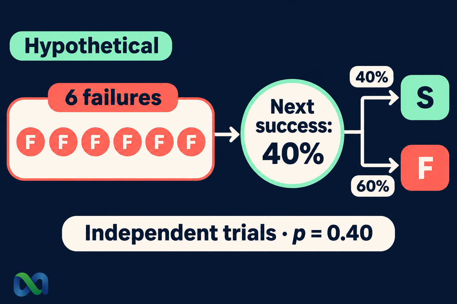
Consider a hypothetical process with a known 40% success probability on every independent trial. Six failures do not use up a failure allowance. The next trial still has a 40% success probability and a 60% failure probability. That conclusion follows from the model; it is not a claim about all financial data points.
You can also make the opposite mistake by treating a run of successes as proof that the next independent outcome is more likely to succeed. Both errors substitute the appearance of the sequence for an explanation of its probability.
The Formula Behind the Mistake
Let S mean success on the next trial, and let H describe the observed history. If the next trial is independent of that entire history, then:
P(S given H) = P(S) = p
For n independent trials with the same success probability p, the chance of a stated run of n failures is:
P(n failures) = (1 − p)^n
These formulas answer different questions. The first concerns the next outcome after the history is known. The second concerns a complete sequence stated before it occurs.
With p = 0.40, six failures have probability 0.60^6 = 4.6656%. Seven failures have probability 0.60^7 = 2.79936%. Once the first six failures are observed, the conditional probability of one more failure is 2.79936% divided by 4.6656%, which is 60%.
The rarity of the full seven-trial sequence is not the chance of its last outcome after the first six are known. Read the conditional probability guide for the denominator change that makes this distinction explicit.
Worked Example: Six Failures Do Not Make Success Due
Suppose you plan 10 hypothetical independent trials, each with p = 0.40. Before starting, the chance of at least one success is:
1 − 0.60^10 ≈ 99.40%
Now suppose the first six trials fail. There are four trials left. The chance of at least one success in those remaining trials is:
1 − 0.60^4 = 87.04%
| Question | Probability |
|---|---|
| Success on trial seven | 40.00% |
| A success in the next four | 87.04% |
| A success in 10 new trials | 99.40% |
The third row starts a new 10-trial calculation. It is not the chance of recovering within the four trials remaining in the original plan. Resetting the label on the plan does not reset the number of opportunities available.
None of these chances measures profitability. A “success” might pay too little relative to the cost of the unsuccessful outcomes. To evaluate an actual decision, define its payoff and use the expected value formula, including the costs that apply to that decision.
Why the Law of Large Numbers Does Not Promise a Rebound
The law of large numbers describes convergence of averages under suitable assumptions. It does not require future data points to reverse previous deviations.
In the hypothetical 40% process, imagine six initial failures followed by 100 fresh independent trials. The expected number of successes in those next 100 trials is 40. The expected overall success fraction across all 106 trials, conditional on the initial failures, is therefore 40/106 ≈ 37.74%.
That fraction is closer to 40% than the initial zero out of six. The improvement can happen through dilution of the early data points, without raising the next trial's success probability above 40%.
The realized fraction can still move farther away before it moves closer. A mathematical convergence result supplies neither a deadline nor a guarantee for a finite account. Limited capital, dependence, and changing probabilities can make a strategy's actual path very different from a textbook sequence.
When Earlier Outcomes Really Can Change a Forecast
The independence assumption is a condition to examine, not a slogan to apply to every chart. Earlier outcomes can be informative when probabilities are unknown, conditions change, or data points share a cause.
Suppose you do not know whether a forecasting process is well calibrated. A long sequence of misses may be evidence that its probability estimates are wrong. Revising those estimates can be reasonable. The reasoning is that the sequence provides information about the model, not that success has become due.
Similarly, an economic release can change expectations for a later policy decision. These events are not interchangeable draws from a bag of independent outcomes. A shared inflation trend, common data source, or changing policy reaction can connect them.
Research on perceived independence discusses how judgments about sequences can go wrong when people misunderstand the relationship between outcomes. A useful practical test is to name the new information and explain how it changes the probability. “It has happened too often” is not enough by itself.
The Financial Cost of Chasing a Reversal
Consider a purely hypothetical contract that pays $1 on success and $0 otherwise. Assume the true success probability is known to be 50%, the purchase price is $0.55, and there are no extra charges. Expected net profit per contract is:
0.50 × $1 − $0.55 = −$0.05
Buying after a losing streak does not change that calculation if the probability and price remain unchanged. Increasing the quantity multiplies both the exposure and the expected loss.
A doubling schedule also creates a funding problem. Quantities of 1, 2, 4, 8, 16, and 32 add up to 63 units. The next quantity is 64 units. This arithmetic describes quantities, not a universal recovery system: actual recovery depends on purchase prices, payouts, fees, and position limits.
Before increasing exposure, separate two decisions. Has new evidence improved the expected value at the current price? And can the account tolerate the full loss? A desire to erase previous losses answers neither question. The risk-reward ratio guide explains another part of the payoff calculation, but a favorable-looking ratio alone does not establish a favorable probability.
A Better Review Process for a Losing Streak
Start by recording the event definition, forecast probability, entry price, quantity, and result for each decision. Separate positions on the same event from genuinely different events. Ten purchases of one contract do not provide 10 independent data points of its settlement.
Then review the forecast without reference to the amount you want to recover. Identify information that was available at entry and information learned afterward. This prevents later knowledge from making an earlier decision appear more predictable than it was.
Check whether losses cluster by event type, data source, or time period. Such clustering may reveal dependence or a model weakness. It is a reason to investigate, not proof of any specific explanation. A larger sample can improve an analysis only when the data points and measurement process remain suitable.
Finally, write the action rule before the next result: what evidence would change the forecast, what price would make entry acceptable, and what exposure limit applies? A rule tied to evidence and price is easier to audit than a rule tied to whether the last outcome felt unfair.
Frequently Asked Questions
Does a long losing streak make the next outcome more likely to succeed?
Not when the next trial is independent and its success probability is known and unchanged. A streak can still prompt a sensible check of whether those assumptions are true. That check differs from assuming a compensating win must arrive.
Is the gambler's fallacy the same as regression to the mean?
No. Regression to the mean concerns less extreme conditional predictions when repeated measurements are imperfectly related. It does not create a debt that the next result must repay. Neither concept guarantees that a falling asset will recover.
Can historical results ever help forecast the next event?
Yes. Historical data points can help estimate unknown probabilities or reveal changing conditions. Explain the information link and its limitations rather than treating every sequence as independent or every streak as meaningful.
Does doubling a position remove the fallacy?
No. Position size does not alter an independent event's probability. A doubling schedule can reach capital or position limits quickly, and its recovery arithmetic depends on the actual payoff structure.
How should I use this in prediction markets?
Read the event rules, distinguish repeated positions from independent outcomes, update probabilities only for defensible information, and compare those estimates with the current all-in price. Evaluate the next decision on its own economics rather than its ability to repair the previous one.
