


Geometric Distribution: Formula and First-Success Examples

A geometric distribution models the number of independent trials needed to obtain the first success when each trial has the same success probability. In the convention used here, the count includes the successful trial and begins at one.
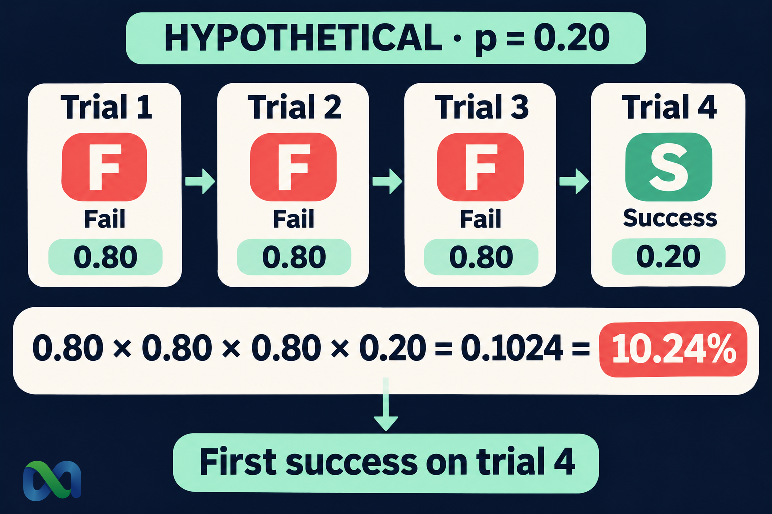
If each hypothetical trial has a 20% success probability, the chance that the first success occurs on trial four is 10.24%. The chance of obtaining at least one success within five trials is 67.232%. Those are different questions, and neither means a success must occur by the fifth trial.
This guide explains the formula, expected waiting count, cumulative probabilities, and the alternative convention that counts failures before success. All examples describe a mathematical experiment rather than actual prediction-market results or a trading recommendation.
What Is a Geometric Distribution?
Let X count the trial on which the first success occurs. The geometric model assumes two outcomes per trial, independence across trials, and a fixed success probability p with 0 < p ≤ 1. The possible values of X are 1, 2, 3, and so on.
“Success” is a label for the event being counted. It might mean an indicator meets a prespecified condition. It does not have to mean that a position is profitable or a forecast is correct. Define it before measuring the waiting count.
SciPy’s geometric-distribution documentation uses the first-success trial convention and gives its probability mass function. Other tools and textbooks can count failures instead, shifting the support to zero, one, two, and so on.
The assumptions matter more than the label. If a trial’s probability changes after an announcement, or if outcomes share a common cause, a single geometric model may not fit. Repeating a similar-looking event does not establish independence or a common p.
The Geometric Distribution Formula
For the first success on trial k, the first k − 1 trials must fail and trial k must succeed:
P(X = k) = (1 − p)^(k − 1) × p, for k = 1, 2, 3, …
Independence lets those probabilities be multiplied. If p = 0.20 and k = 4, the required sequence is failure, failure, failure, success. Its probability is:
0.80³ × 0.20 = 0.1024 = 10.24%
There is no binomial combination term because the first-success condition fixes the sequence: every preceding trial must fail. A success on trial two would mean that the first success was not on trial four.
The model assumes trials can continue without a fixed upper limit. A plan that stops permanently after five attempts introduces a limit on what can be observed. You can still calculate success by five, but the chance of no success within the plan must remain visible.
Worked Example: A 20% Success Probability
Assume p = 0.20 on every independent trial. The probability that the first success arrives on each of the first five trials is:
| Trial | Sequence | Probability |
|---|---|---|
| 1 | S | 20.000% |
| 2 | FS | 16.000% |
| 3 | FFS | 12.800% |
| 4 | FFFS | 10.240% |
| 5 | FFFFS | 8.192% |
In the table, F denotes failure and S denotes success.
The probabilities decline because later first successes require a longer uninterrupted sequence of preceding failures. The success probability on an individual trial remains 20%. A declining first-success probability does not mean each new trial becomes less likely to succeed.
Add the first five rows to get 67.232%. The remaining 32.768% corresponds to no success in the first five trials. It includes all possible first-success times after trial five.
The example deliberately assumes the probability instead of estimating it. Applying the calculation to real observations requires evidence about p and the structure of the trials. Our independent-events guide explains why related markets should not automatically be treated as separate independent experiments.
Cumulative and Tail Probabilities
The probability of no success through trial k is the probability that all k trials fail:
P(X > k) = (1 − p)^k
Taking the complement gives the probability that the first success occurs by trial k:
P(X ≤ k) = 1 − (1 − p)^k
For five trials at p = 0.20, these become 0.80⁵ = 0.32768 and 1 − 0.80⁵ = 0.67232. The cumulative result includes success on trial five. “Before trial five” includes only trials one through four and has probability 59.04%.
The probability of a first success after trial three but by trial five is P(X > 3) − P(X > 5) = 0.80³ − 0.80⁵ = 18.432%. This equals the sum of the probabilities for trials four and five.
Write the event in plain language before selecting a formula. “On,” “by,” “before,” and “after” define different sets of integer outcomes. A one-trial indexing mistake can produce a materially different result.
Mean, Variance, and Median
For a first-success count, the expected number of trials is 1/p. The variance is (1 − p)/p², and the standard deviation is its square root. With p = 0.20, the mean is five trials, the variance is 20 trials squared, and the standard deviation is approximately 4.472 trials.
The mean is an average across repeated complete experiments. It is not a deadline, a guaranteed maximum, or the most likely outcome. The most likely first-success time in this example is trial one, even though the expected count is five.
The median is four trials: the chance of success by trial three is 48.8%, and the chance by trial four is 59.04%. Thus four is the first integer at which the cumulative probability reaches at least 50%.
For a 95% cumulative threshold, solve 1 − 0.80^k ≥ 0.95 and round up to an integer. The result is 14 trials. Even that threshold leaves approximately 4.40% probability of no success through trial 14. It is not a promise that a bounded sequence will succeed.
Trials Until Success vs. Failures Before Success
Let Y count only the failures before the first success. Then Y = X − 1. Its possible values start at zero, and its probability formula is P(Y = j) = (1 − p)^j p for j = 0, 1, 2, and so on.
At p = 0.20, the expected number of failures is (1 − p)/p = 4, while the expected total number of trials is five. Subtracting one shifts the mean but does not change the variance or standard deviation.
The University at Buffalo probability demonstration illustrates the trial-number version. When moving between software and a written formula, confirm which version the variable represents before comparing results.
In some software, a geometric variate of zero means success on the first trial because zero failures preceded it. In another function, a returned one means that same event. Both conventions can be correct; mixing them within a calculation creates an error.
Geometric vs. Binomial and Bernoulli Models
A Bernoulli distribution describes the zero-or-one outcome of one trial. A binomial distribution counts successes across a fixed number of comparable independent trials. A geometric distribution counts trials until the first success.
For p = 0.20, “How many successes occur in five trials?” is a binomial question. “On which trial does the first success occur?” is geometric. The probability of at least one success within five trials can be calculated through either model because the events coincide.
The geometric model is also a special case of a negative binomial waiting-count model, with the target number of successes equal to one. Waiting until the third success requires a different formula and a clear counting convention.
Choose the stopping rule before the distribution. If the number of trials is fixed, a first-success model does not replace a complete count analysis. If you stop at the first success, treating the realized trial count as if it had been fixed in advance changes the experiment.
Memorylessness and Financial Limits
Under the geometric assumptions, previous failures do not change the probability of success on the next trial. After 10 failures, the next trial still has probability 20% in the example. A success is not due merely because it has not yet occurred.
The distribution of the additional number of trials until success is also unchanged. Its mean remains five trials. This is a conditional statement under a fixed-p independent model; it does not mean the total number of trials already used disappears from the record.
In real financial research, a long failure sequence may provide evidence that p was estimated poorly or that conditions have changed. Updating the model using new evidence is different from assuming that an independent process must compensate for its history.
The model also says nothing about the cost of waiting or repeating positions. A 20% occurrence probability can coexist with positive or negative economic value depending on price and payoff. Use the expected value formula for that separate calculation, including fees and losses rather than counting occurrences alone.
Spreadsheet Calculation
For the probability of a first success on trial four, an English-language spreadsheet can calculate =(1-0.2)^(4-1)*0.2. For success by trial five, use =1-(1-0.2)^5. Both formulas produce the values shown above without depending on a software-specific geometric convention.
For a cumulative target q, calculate =ROUNDUP(LN(1-q)/LN(1-p),0) when 0 < p < 1 and 0 < q < 1. Handle p = 1 separately: success occurs on trial one with certainty. With p below one, no finite trial count guarantees a success.
Keep the unrounded probability through the calculation. Define success consistently and avoid combining changing trial types into one p without justification. A spreadsheet can verify arithmetic, but it cannot validate the independence or stability assumptions for you.
Frequently Asked Questions
Can the expected trial count be fractional?
Yes. An expectation averages many hypothetical experiments and need not be a possible individual outcome. Every realized first-success count is an integer, while 1/p can be fractional.
Does the distribution require a 50% success probability?
No. Any fixed p in (0, 1] is allowed. The same p must apply to each independent trial under the basic model.
Is a success guaranteed if I keep trying?
For p > 0 under the ideal infinite independent-trial model, the probability of eventually obtaining a success is one. That does not guarantee success within a finite budget, time limit, or sequence of actual trading opportunities.
