


Joint Probability: Formula and Worked Financial Examples

Joint probability is the chance that both events happen. It is written P(A ∩ B), where the middle symbol means the intersection of the events. This asks a different question from at least one event happening, or one event happening given the other. Keeping those questions separate helps you choose the right formula and the right group to count.
Two separate forecasts do not tell you how often two events occur together. A low inflation reading and a rate cut can share a cause. Multiplying their standalone chances assumes independence. You need a reason for that assumption before you use it. Different names, dates, or charts do not by themselves show that the events are independent.
This guide uses one coherent hypothetical example to work out joint, marginal, and conditional probabilities. It also checks the range of possible answers, shows a spreadsheet method, and explains how dependence affects a combined payoff. All probabilities and payoffs are teaching inputs. They are not live Macro Markets quotes, forecasts, or product descriptions. The event definitions and their shared information come before the math.
What Is Joint Probability?
Define event A and event B within the same probability model. The joint event A ∩ B occurs only when both are true. Its probability cannot exceed either single event's probability because the intersection is contained within each event.
For a financial example, A could be a precisely defined rate cut at a stated policy meeting, while B could be a stated inflation release falling below a stated threshold. Their sources, deadlines, and measurement definitions must be clear before their chances can be combined.
OpenStax's probability rules express the general multiplication rule using a conditional probability. That rule works for dependent events as well as independent events.
The events do not need to happen at the same moment. “Both occur” can refer to two events at different stated dates within one model. What matters is that the definitions and information set are consistent. A later event may be affected by information revealed when the earlier event occurs.
Joint Probability Formula
The general multiplication rule is:
P(A ∩ B) = P(A) × P(B given A)
Equivalently, P(A ∩ B) = P(B) × P(A given B). The conditional form requires a positive probability for the event being conditioned on when that conditional probability is calculated by division.
If A and B are independent, P(B given A) equals P(B), and the rule simplifies to:
P(A ∩ B) = P(A) × P(B)
That simplification is a special case, not the definition of joint probability. Shared economic drivers, overlapping event definitions, or a common data source can make it unsuitable.
The conditional probability guide explains the “given” part of the general formula. The independent events guide explains the extra condition needed to replace the conditional probability with a marginal one.
Worked Example: Two Events With an 18% Joint Probability
Assume a hypothetical model assigns P(A) = 40%, P(B) = 30%, and P(B given A) = 45%. The joint probability is:
P(A ∩ B) = 0.40 × 0.45 = 0.18 = 18%
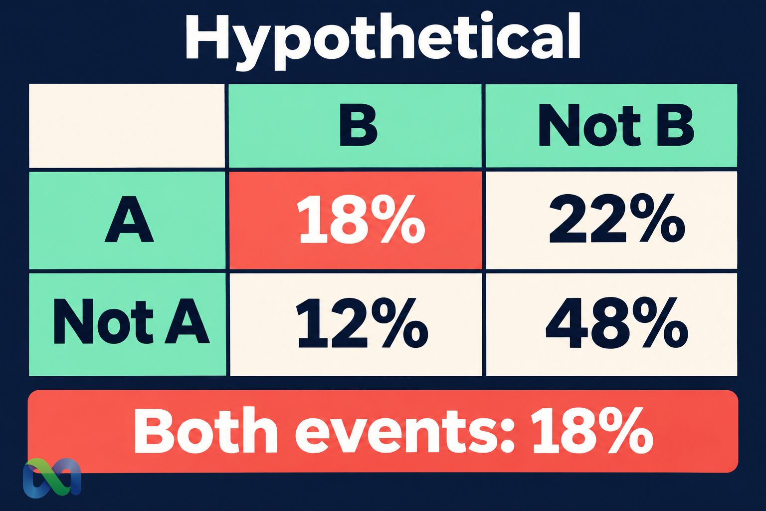
For a natural-frequency representation, imagine 100 hypothetical equally weighted cases. Eighteen contain both events. Another 22 contain A without B, 12 contain B without A, and 48 contain neither.
| Case | B | Not B |
|---|---|---|
| A | 18% | 22% |
| Not A | 12% | 48% |
All four cells add to 100%. Adding across the first row gives P(A) = 40%. Adding down the first probability column gives P(B) = 30%. The joint probability is the upper-left cell, 18%.
This table is a complete joint distribution of two binary indicators under the stated model. It is internally consistent, but internal consistency alone does not validate the assumed probabilities against real data.
The events are not independent: 40% × 30% = 12%, which differs from the stated joint probability of 18%. Assuming independence would understate the chance of both events in this constructed example.
Joint, Marginal, and Conditional Probability
A marginal probability describes one event without restricting the population to the other event. In the example, the marginal probabilities are 40% for A and 30% for B.
A joint probability uses the original population and counts cases where both events occur. That gives 18 out of 100 hypothetical cases, or 18%.
A conditional probability changes the denominator. Among the 40 cases where A occurs, 18 also contain B, so P(B given A) = 18/40 = 45%. Among the 30 cases where B occurs, 18 also contain A, so P(A given B) = 18/30 = 60%.
The 45% and 60% answers are both correct. They use different conditioning populations. Swapping them without changing the denominator is a common error.
The Bayes' theorem guide explains how to reverse the direction of conditioning using the marginals. The example also shows why an event's standalone probability is not the same as its probability after related information becomes known.
Both Events vs. Either Event
The chance of A or B, including the possibility of both, uses the addition rule:
P(A ∪ B) = P(A) + P(B) − P(A ∩ B)
For the example, 40% + 30% − 18% = 52%. Adding the marginals without subtracting the overlap would count the 18% intersection twice.
The chance of neither event is the complement, 100% − 52% = 48%. The chance that exactly one event occurs is 22% + 12% = 34%. These are three distinct questions: both, at least one, and exactly one.
The distinction becomes economically important when a payoff depends on a combination of events. A hypothetical payoff triggered by both events does not have the same probability as one triggered by at least one event. Read the exact payoff condition before calculating.
For mutually exclusive events, the intersection is zero and addition simplifies. But different events are not automatically mutually exclusive. A rate cut and a low inflation reading can both occur under a coherent event definition.
Bounds When You Know Only the Marginal Probabilities
Two marginal probabilities do not determine a unique joint probability. They do impose the bounds:
max(0, P(A) + P(B) − 1) ≤ P(A ∩ B) ≤ min(P(A), P(B))
With marginals 40% and 30%, the joint probability can range from 0% to 30%. Independence gives one admissible value, 12%, but the marginals alone do not establish that value.
At the lower bound, no case contains both events. At the upper bound, every B case also contains A. The hypothetical 18% joint lies between those extremes and implies positive association between the binary indicators.
These bounds can identify impossible inputs. A proposed 35% joint probability would exceed the 30% marginal probability of B. No adjustment to conditional language can make that combination valid; at least one assumption must change.
When there is insufficient evidence about dependence, report a justified range or test alternative joint assumptions instead of silently selecting the independent value.
How Dependence Changes a Combined Payoff
Imagine two hypothetical $1-or-$0 settlement payments, one tied to A and one tied to B. Let their indicators be IA and IB. Expected total payout is E(IA + IB) = 0.40 + 0.30 = $0.70, regardless of dependence, under these marginal assumptions.
The variance does depend on the joint probability. The indicator covariance is:
Cov(IA, IB) = 0.18 − (0.40 × 0.30) = 0.06
Their single variances are 0.24 and 0.21. Total-payout variance is therefore 0.24 + 0.21 + 2 × 0.06 = 0.57 dollars squared. Under independence with the same marginals, it would be 0.45 dollars squared.
This is a teaching calculation, not a description of an available combined product. Purchase prices, costs, event rules, and execution risks would be needed to evaluate net profit. The covariance guide explains how the cross term enters a portfolio variance calculation.
Estimate Joint Probability From a Complete Dataset
For 100 complete hypothetical paired data points, store A as a zero-or-one indicator in A2:A101 and B in B2:B101. Both columns must refer to the same cases, using event information available under a consistent observation rule.
To calculate the fraction where both equal one, use this English Excel formula:
=COUNTIFS(A2:A101,1,B2:B101,1)/100
If 18 paired cases contain both events, the result is 0.18. Check row alignment and verify that all 100 pairs contain valid zero-or-one values. A fixed denominator is wrong if cases are missing or excluded; first define the valid paired population.
An observed fraction is an estimate, not a known future probability. Small samples, repeated exposure to one event, selection bias, and changing conditions can all affect its interpretation. Retain the full four-cell table so that marginal totals and missing data can be audited.
Frequently Asked Questions
Is joint probability always the product of two probabilities?
It is the product of one marginal and the appropriate conditional probability. Multiplying two marginals is valid only when the events are independent.
Can joint probability exceed a marginal probability?
No. Both events occurring is a subset of either event occurring. The joint probability cannot exceed the smaller marginal probability.
Does a positive joint probability mean independence?
No. Independence requires the joint probability to equal the product of the marginals. The example has an 18% joint probability compared with a 12% independent benchmark.
Does correlation supply the entire joint distribution?
Not in general. For two binary indicators with known nondegenerate marginals, their correlation determines their covariance and joint probability when the inputs are valid. For general continuous variables, marginals and one correlation number do not specify the full joint distribution.
