


Linear Regression: Formula and Worked Financial Examples

Linear regression models a numeric response as a function of one or more predictors. In the simple straight-line case, it estimates an intercept and a slope, producing a fitted value for each predictor value. The gap between an observed response and its fitted value is called a residual.
In financial research, a line can help describe an association between a signal and a return. It does not by itself show causation, calibrated forecasts or a profitable strategy. Start by defining the data points, units and question the model is meant to answer.
The Simple Linear Regression Equation
For one predictor x, write the model as:
y = intercept + slope × x + error
The fitted line omits the unobserved error term and uses estimated coefficients. Its output is a modeled conditional mean, not a promise that every data point will equal that value.
The slope describes the fitted change in y associated with a one-unit increase in x. The intercept gives the fitted value when x is zero. That zero may lie outside the observed range, so an algebraically valid intercept does not always have a useful standalone interpretation.
The NIST introduction to linear least squares also explains a broader point: linear refers to the parameters. A model can include a squared predictor and still be linear in its coefficients. This guide focuses on a straight line so that the calculation remains transparent.
What Least Squares Minimizes
Ordinary least squares selects coefficients that minimize the sum of squared residuals. If a prediction misses a data point by two units, it contributes four squared units to that objective. Large residuals thus receive large weight.
For one predictor and an intercept:
Slope = sum of [(x − mean x)(y − mean y)] / sum of [(x − mean x)²]
Intercept = mean y − slope × mean x
The denominator must be positive. If every x value is the same, the sample contains no variation from which to estimate a separate slope using this formula.
The NIST least-squares derivation provides the estimator formulas. Their connection to covariance helps explain why the sign of the fitted slope follows the direction of the sample association.
Worked Example: A Signal and a Return
Consider five hypothetical data points. The predictor is an illustrative economic signal measured in index units. The response is the following period's return, recorded as percentage values. These small teaching inputs are not actual market data or a fitted Macro Markets strategy.
| Signal x | Return y |
|---|---|
| 1 | 2% |
| 2 | 4% |
| 3 | 5% |
| 4 | 4% |
| 5 | 5% |
Using the numeric return values 2, 4, 5, 4 and 5, mean x is 3 and mean y is 4. The numerator in the slope calculation is 6, while the denominator is 10. The fitted slope is thus 0.6.
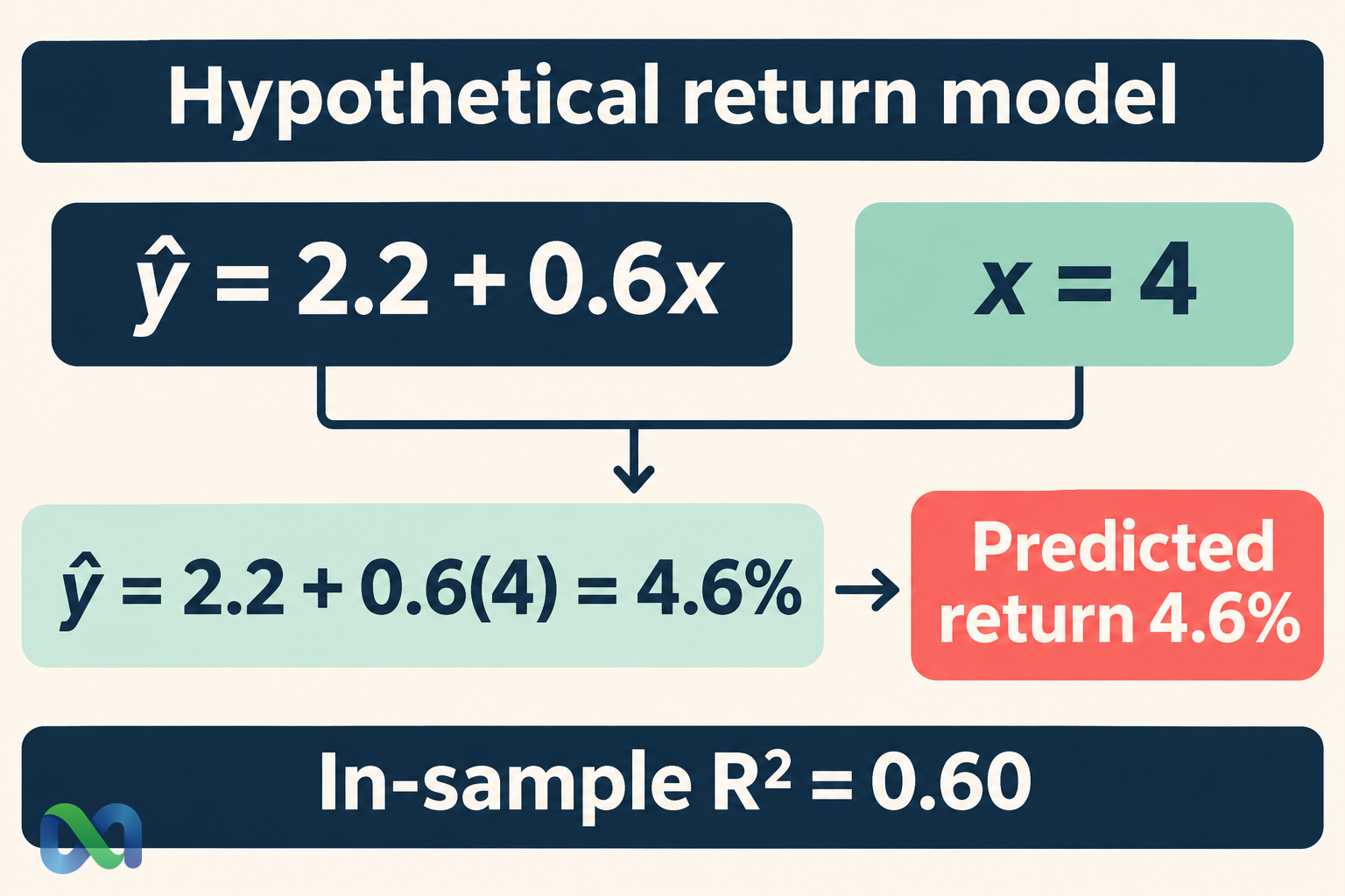
The intercept is 4 − 0.6 × 3 = 2.2. The fitted equation is:
Predicted return, in percent = 2.2 + 0.6 × x
For x = 4, the fitted return is 4.6%. The observed return in that row is 4%, so the residual is 4 − 4.6 = −0.6 percentage points. A positive predictor value does not remove uncertainty around the fitted response.
The slope means a one-unit increase in the signal is associated with a fitted increase of 0.6 percentage points in return. It does not mean the return multiplies by 0.6 or rises by 60%. Keep percentage values and percentage-point differences distinct.
Residuals and R-Squared
The fitted values for the five data points are 2.8%, 3.4%, 4.0%, 4.6% and 5.2%. The residuals, in percentage points, are −0.8, 0.6, 1.0, −0.6 and −0.2.
Their squared sum is 2.4. The corrected total sum of squares, computed around the sample mean return of 4%, is 6. With this fitted-intercept setup:
R-squared = 1 − residual SS / total SS = 1 − 2.4 / 6 = 0.60
| Quantity | Result |
|---|---|
| Slope | 0.6 |
| Intercept | 2.2 |
| Residual SS | 2.4 |
| R-squared | 0.60 |
Here, 60% of the sample's corrected variation is accounted for by the fitted line in the least-squares decomposition. It does not mean that 60% of trades will win, that predictions are 60% accurate or that 60% of the causal explanation has been discovered.
The correlation-coefficient guide describes another summary of association. In a simple ordinary least-squares regression with an intercept, R-squared equals the squared sample correlation. That relationship depends on the model setup and should not be generalized to every regression output.
Association Does Not Establish a Cause
A fitted relationship can reflect a common driver, selection effects, timing or an omitted variable. Adding more digits to a coefficient does not distinguish those explanations.
For example, the economic signal and return in a real study could both respond to another release. A positive coefficient would summarize their observed association under the fitted model. A causal interpretation would require a design and assumptions that justify the stronger claim.
Timing is especially important in forecasting. Predictor values must have been available before the response being predicted. Revised economic data, future classifications or information selected after the outcome can make a historical fit look more useful than it would have been at the decision time.
Regression to the mean is also a separate concept. It describes what can happen after selecting extreme measurements when repeated measurements are imperfectly correlated. Fitting a line and predicting a reversal are not interchangeable operations.
Check the Model, Not Just the Coefficient
Inspect the residuals for patterns that suggest the straight-line mean is inadequate. A curve, changing spread, clusters or unusual data points can show that the model misses important structure. A single R-squared value cannot show all those features.
The assumptions needed depend on the claim. Estimating a descriptive best-fitting line requires less than making a standard statistical confidence statement about a population parameter. Classical inference typically introduces assumptions about the errors, their relationship to predictors, dependence and variance.
Normal errors can justify specific small-sample inference procedures, but normality is not required just to compute least-squares coefficients. State what your inferential method assumes rather than describing every regression as the same procedure.
Financial time series can contain dependence and changing conditions. A method suitable for independent data points may need adjustment when returns overlap or errors are correlated. The five-row example illustrates arithmetic; it is not enough data to show a reliable forecasting model.
Prediction, Uncertainty and Extrapolation
The line predicts 5.8% at x = 6. That is a correct substitution into the fitted equation, but x = 6 lies outside the example's observed range of 1 through 5. The extra step depends on extending a relationship beyond the data used to fit it.
Even within the observed range, a fitted mean and an individual future outcome are different targets. A confidence interval for a mean response and a prediction interval for a new data point answer different questions. Their widths depend on the method and assumptions.
The confidence-interval guide explains why uncertainty needs a stated procedure and interpretation. Reporting a point forecast without those limits can make a modest descriptive fit look more decisive than it is.
Assess forecasting performance on suitable unseen data. In time-ordered settings, preserve the information order when splitting or validating data. A model assessed on the same data points used to choose its predictors can benefit from selection that a new forecast will not enjoy.
A Useful Reporting Checklist
State the response, predictors, units, sampling period and inclusion rules. Show the fitted equation and enough of the calculation or data for another person to reproduce it.
Then report residual behavior, uncertainty and the review design. Distinguish a fit that describes historical data points from a claim about future predictions. Explain how unusual records, missing data and revised information were handled.
Finally, connect the output to the actual question. A return forecast does not alone show an executable advantage after spread, fees and other costs. A modeled relationship can inform analysis while remaining an uncertain component of a broader decision.
Frequently Asked Questions
Does linear regression always produce a straight line?
No. Linear means linear in the coefficients. This guide uses the simple straight-line case, but models with transformed predictors can also be linear in their parameters.
Does a high R-squared prove a model is useful for trading?
No. It is a feature of the fitted sample and model. Causation, information timing, future validation and financial implementation need separate examination.
Is the slope a probability?
Generally no. Its units depend on the response and predictor. In the example it is a change of 0.6 percentage points of fitted return per signal unit.
Can I use the fitted line outside the data range?
You can compute an extrapolated value, but its reliability requires more justification. A mathematical output does not show that the historical relationship continues outside the observed range.
