


Regression to the Mean: Meaning and Financial Examples
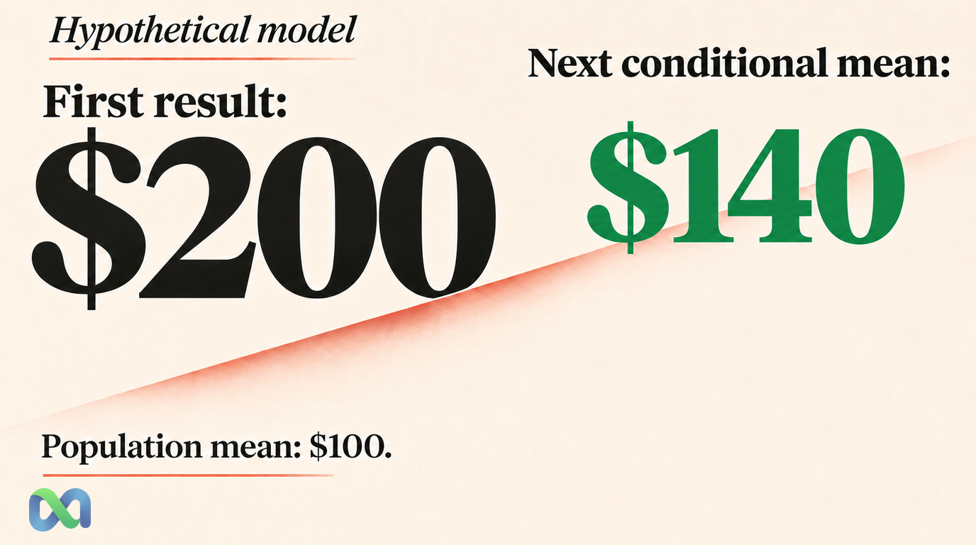
Regression to the mean describes a pattern in repeated measures. Take a group whose first results were far from the mean. When the two sets of results are linked but do not match perfectly, the model tends to predict less extreme next results for that group. It does not say that each case must reverse or that a losing asset must recover.
This matters when you review returns. The best recent results can reflect both lasting skill and a run of good luck. The worst can reflect bad luck as well as weak skill. A more normal next result can then look like a change in skill, even when the skill itself did not change.
This guide shows how choosing extreme cases can affect what you see next. It uses a hypothetical model to separate that pattern from cause and effect and from a trading rule. All dollar values are teaching inputs. They are not real returns, forecasts, or results from Macro Markets users.
What Is Regression to the Mean?
Suppose you measure the same group twice. Choose the cases far above the first mean. If the two measures have a positive link that is less than perfect, the next fitted value is closer to the second mean in standardized units. The comparison uses each measure's own mean and spread.
The key word is predicted. Some cases will be more extreme the next time. The statement describes a mean for a group or a fitted forecast. It does not describe a rule that every path must follow.
This pattern does not mean each person has changed. Colorado State University's regression lesson explains why it can arise even if the underlying traits stay the same. The lesson also links the size of the effect to correlation.
Think of a result as two parts: a part that tends to last and a part that changes from one time to the next. An extreme result may include a large dose of good or bad luck. If that short-term part does not repeat, the next result can look more normal. The lasting part need not have changed.
That explanation is a model of how the pattern can arise. It is not proof that every financial performance difference is noise.
The Regression-to-the-Mean Formula
For a simple linear prediction of a second measurement Y from a first measurement X:
Predicted Y = μY + ρ × (σY/σX) × (X − μX)
Here, μX and μY are the means, σX and σY are the standard deviations, and ρ is the correlation. In standardized units, the relationship is:
Predicted zY = ρ × zX
The first expression is the best linear predictor for the full population when the needed means and variances exist. Under a bivariate normal model, it also equals the conditional mean E(Y given X). That term means the mean of Y for a given X. Without that model, the conditional mean need not follow a straight line.
OpenStax's regression-equation reference distinguishes fitted predictions from observed values. The correlation coefficient guide explains the standardized association used in the formula.
For 0 < ρ < 1, the predicted standardized deviation has the same sign but a smaller magnitude than the starting deviation. Raw dollar differences also depend on the relative standard deviations, so a slope below one should not be assumed without checking the scales.
Worked Example: An Extreme Result and Its Next Prediction
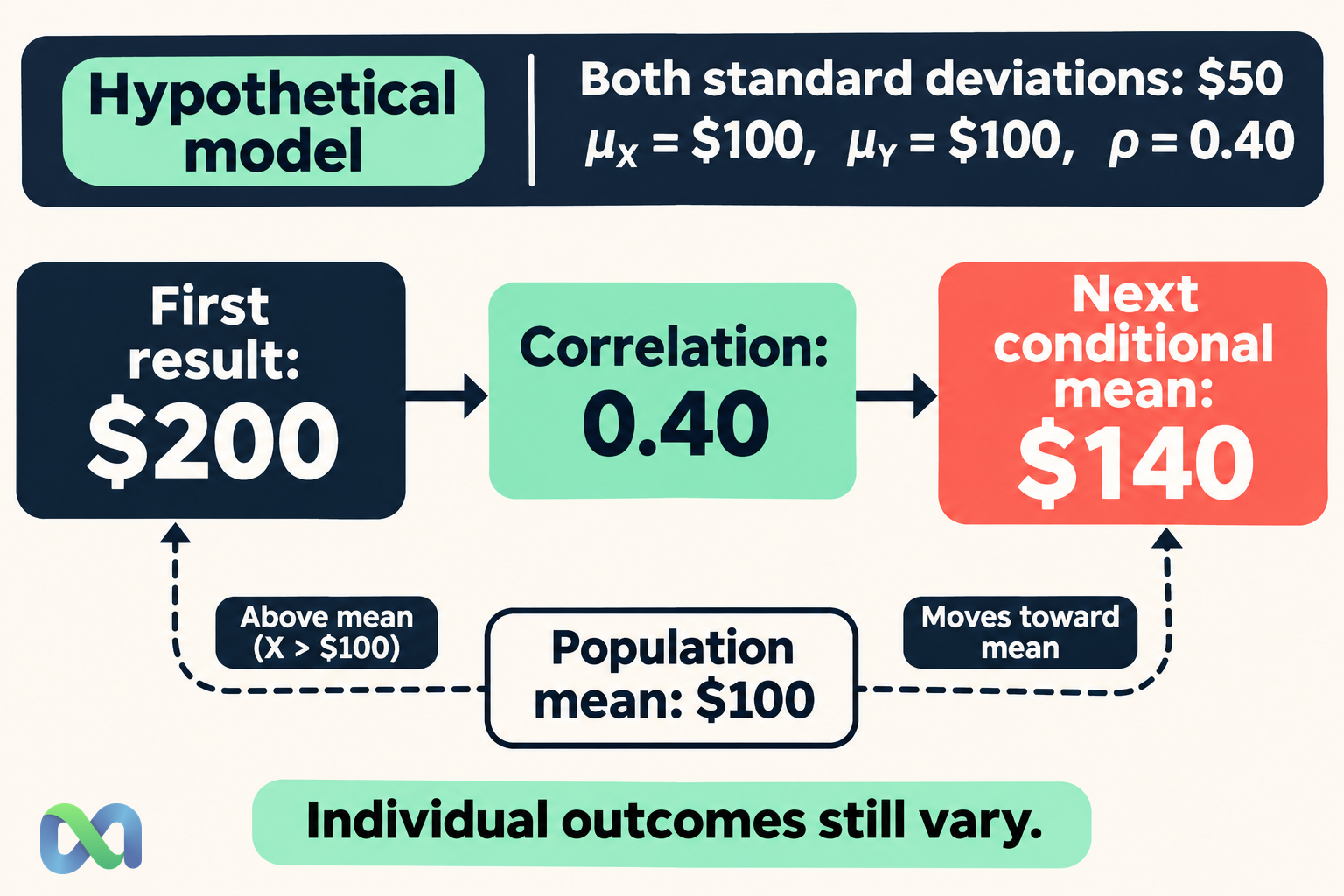
Assume a hypothetical pair of comparable monthly net-profit measurements follows a bivariate normal model. Set both population means to $100, both standard deviations to $50, and correlation to 0.40. These assumptions define a teaching model; no historical returns have been fitted.
Suppose the first measurement is $200. Its standardized value is:
zX = ($200 − $100)/$50 = 2
The predicted second standardized value is 0.40 × 2 = 0.8. Converting back to dollars gives:
E(Y given X = $200) = $100 + 0.8 × $50 = $140
| First result | Predicted next mean |
|---|---|
| $0 | $60 |
| $100 | $100 |
| $200 | $140 |
The high first result is followed by a lower conditional mean, but that mean remains above the population average. The low first result is followed by a higher conditional mean, which remains below average. The model does not predict identical next results for everyone.
For the assumed bivariate normal model, conditional standard deviation is $50 × √(1 − 0.40^2) ≈ $45.83. That large uncertainty remains around the conditional mean. A point prediction of $140 does not imply that $140 is the next realized profit.
Why Selection Changes the Comparison
Imagine reviewing only accounts after a month of very high returns. You chose the group using the same result you now treat as its normal baseline. Some of that high return may reflect conditions that did not last. A more normal next month can then look like a steep decline in skill.
Now choose accounts after their worst recent month. A more normal next month can look like a turnaround even if no new rule helped. That improvement alone does not show cause and effect. The study needs a way to tell the effect of the new rule from selection and other changes.
In the hypothetical model, the full group still has a second-month mean of $100 and standard deviation of $50. The fitted means move inward, but the real results need not form a tighter group. Each result also has a residual: its gap from the fitted mean. Those residuals add spread back to the actual results.
This distinction prevents a common reporting error: describing a narrowing set of model predictions as proof that actual outcomes have become safer. The standard deviation guide explains the difference between the spread of observed outcomes and a summary of their central tendency.
Regression to the Mean vs. a Reversal Being Due
A reversal-being-due argument says an outcome must compensate for earlier results. Regression to the mean requires no compensation account. It is a statement about a conditional expectation or a fitted prediction under a stated relationship.
For a known independent process, correlation between successive measurements can be zero. The next prediction is then its population mean regardless of the first result. A below-average first observation does not force the next observation above average to repair it.
In financial markets, successive data points may be dependent and probabilities may change. Those features require an explicit model. They do not justify moving directly from “the price fell” to “the expected return is now positive.” The independent events guide helps identify when earlier outcomes do or do not supply information about a later event.
Always ask what is regressing: a performance estimate, an observed level, a return, or a forecast error. A relationship estimated for one of those variables does not automatically transfer to the others.
Regression to the Mean vs. a Trading Strategy
A mean-reversion strategy makes a claim about predictable future price behavior after a stated deviation. That claim needs a definition of the relevant mean, an estimation period, an entry and exit rule, and evidence that survives costs and out-of-sample evaluation.
The pattern alone supplies no entry price or exit rule. A price can stay low. A business can worsen, and the market's long-run level can shift. Even if a model describes future results well, a trade at the available price may still lose money on average.
The expected value formula guide connects outcome probabilities with payoffs and costs. Use that framework before treating a statistical pattern as an economic opportunity.
For a prediction market, a settlement probability can change because new information arrives. A contract trading at a low price is not automatically an extreme measurement drawn from a stable repeated-measurement model. Its event rules, deadline, and information set determine which comparisons are defensible.
How to Evaluate Performance Without Overstating Improvement
Define the review cohort before observing the outcomes whenever possible. If you select only recent winners or losers, disclose that selection and compare them with a relevant group selected in the same way.
Keep the measurement consistent. A gross return cannot be compared directly with a net return after fees, and a short event window cannot be treated as a complete year. Changes in exposure can also change the scale of results, making an apparent improvement difficult to interpret.
For an intervention, such as a new forecasting process, use an appropriate control or comparison design. A before-and-after chart alone can combine regression to the mean, changing market conditions, altered risk, and the intervention itself.
Finally, retain unsuccessful forecasts and account for uncertainty in estimated correlations and means. The hypothetical example above treats its parameters as known. Real estimates carry sampling error, and a changing regime can invalidate the relationship. The confidence interval guide explains one way to describe estimation uncertainty under suitable assumptions.
Frequently Asked Questions
Does regression to the mean mean the next result must improve?
No. It concerns a conditional prediction or group pattern. Single outcomes can become more extreme. The direction and size of a prediction depend on the relationship and scales being modeled.
Is regression to the mean evidence that a training program worked?
Not by itself. If participants were chosen because their starting measurements were unusually poor, some later improvement can occur without the program. A suitable comparison design is needed to estimate a causal effect.
Can regression to the mean occur when nothing fundamentally changes?
Yes. A stable underlying component combined with temporary measurement noise can produce the pattern. This is one reason a selected extreme observation may be a poor baseline for evaluating change.
Does a correlation of 0.40 mean 40% of the prior profit repeats?
No. In the standardized linear prediction, 40% of the deviation from the first mean carries into the predicted deviation from the second mean. The dollar formula also depends on both means and standard deviations.
Is buying a falling asset an application of regression to the mean?
Only if a defensible model supports the relevant forecast, and even then profitability requires a separate calculation. A fall in price alone does not establish a stable mean, a reversal mechanism, or positive expected net profit.
