


Logistic Regression: Formula and Binary Forecast Examples

Logistic regression models the probability of an outcome that belongs to a defined category. In the binary case, the outcome is coded as 1 or 0, and a logistic function maps a predictor score into a probability between zero and one.
That makes it relevant to event forecasting, where a question may resolve yes or no. The model's probability is still conditional on its inputs, coefficients and assumptions. A bounded number is not by itself a well-calibrated estimate or an executable trading advantage.
From a Predictor Score to a Probability
For one predictor x, start with a linear score z:
z = intercept + slope × x
Then apply the logistic function:
p = 1 / [1 + exp(−z)]
The function changes the score into a value strictly between zero and one for finite z. A score of zero gives p = 0.50. Positive scores give probabilities above 0.50, while negative scores give probabilities below it.
The Stanford CS229 notes on classification develop this model for binary labels. The scikit-learn discussion of logistic regression also distinguishes its classification role and describes implementation choices such as regularization. Name the fitted procedure when presenting an actual model.
The response is categorical even though the model outputs a probability. A system can later apply a decision threshold to that probability, but estimating a probability and choosing an action are separate steps.
Worked Example: A Hypothetical Event Signal
Suppose an event has a fixed yes-or-no resolution rule and horizon. Let x be an illustrative signal measured in index units. Choose the following coefficients purely to demonstrate the transformation:
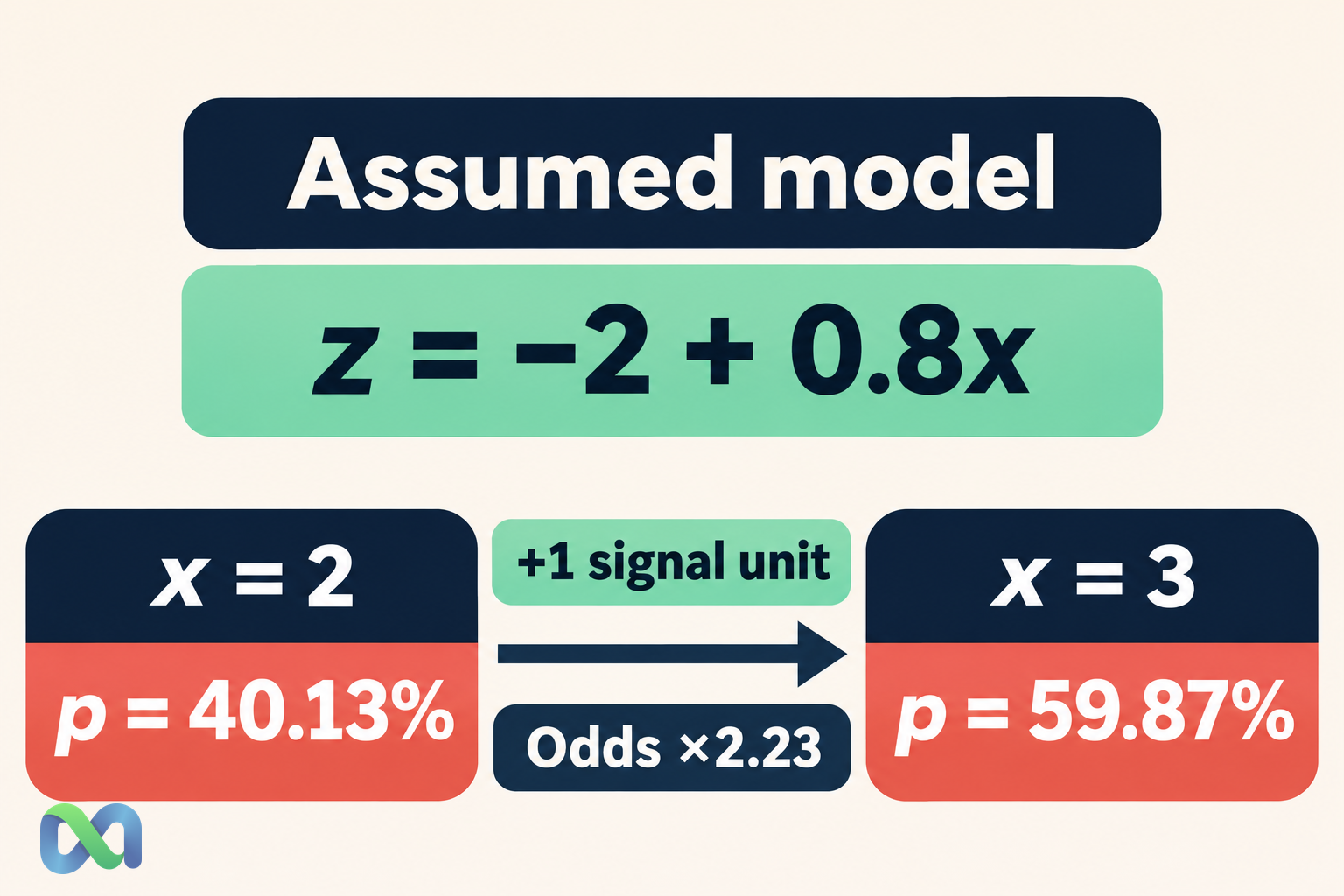
z = −2 + 0.8 × x
These coefficients are assumed, not estimated from a training sample. The example thus shows how a stated model behaves, not evidence that this signal predicts a real event.
At x = 3, the score is −2 + 0.8 × 3 = 0.4. The matching model probability is:
p = 1 / [1 + exp(−0.4)] ≈ 0.5987
That is about 59.87%. At x = 2, the score is −0.4 and the probability is about 40.13%. The one-unit increase changes probability by about 19.74 percentage points in this part of the curve.
| Signal x | Model probability |
|---|---|
| 0 | 11.92% |
| 1 | 23.15% |
| 2 | 40.13% |
| 3 | 59.87% |
| 4 | 76.85% |
| 5 | 88.08% |
The same one-unit increase has a smaller probability effect near either end of the curve. A constant coefficient in the score does not create a constant percentage-point change in probability.
The model also does not tell us that a specific future event is 59.87% likely just because we can compute that value. To support such an interpretation, the inputs, fitted coefficients, population and performance of the model need empirical assessment.
Odds Ratios Are Not Probability Ratios
Odds are p / (1 − p). In a simple logistic model, the log of those odds equals z. A one-unit increase in x thus multiplies the model odds by exp(slope).
For the assumed slope of 0.8:
Odds ratio per signal unit = exp(0.8) ≈ 2.2255
This does not mean probability increases by 122.55%. The probability change depends on the starting point. In the worked example, the move from x = 2 to x = 3 changes probability from about 40.13% to 59.87%.
With several predictors, a coefficient describes a change while the other included predictors are held fixed within the model. That qualification matters when predictors are related. It is not a claim that the variable can be independently changed in the real world.
The conditional-probability guide helps explain what it means to condition on information. The model conditions on its recorded predictors; omitted information and measurement errors can still matter.
How Real Coefficients Are Estimated
An actual binary training sample contains predictor values and observed labels. A fitting procedure selects coefficients according to an objective, commonly a likelihood-based loss with any stated penalty or regularization.
For a labeled data point y that equals 0 or 1, the probability assigned to its observed result is p when y = 1 and 1 − p when y = 0. A log-loss objective penalizes assigning very low probability to what actually occurs.
Regularization can constrain coefficients and change the fitted result. Choices about features, penalties, weights and tuning belong in the model description. Two programs both called logistic regression need not produce the same coefficients if their settings differ.
Data quality comes first. The target label must match a stable event definition, and predictor values must have been available at the intended forecast time. A model trained with later information can perform impressively in a historical file without offering the same information advantage in practice.
Sample construction matters too. An artificially balanced training set can differ from the population where predictions will be used. Observed label frequencies, sampling weights and any probability adjustment should be documented rather than silently assuming the training mix is representative.
Calibration and Discrimination Answer Different Questions
A model can rank higher-risk cases above lower-risk cases while assigning inaccurate probability levels. Ranking performance is often called discrimination. Calibration concerns agreement between assigned probabilities and observed frequencies under a suitable review design.
For example, a set of cases forecast near 60% should not be declared well calibrated just because more than half occurred. Assess how closely the observed frequency agrees with the forecast range, accounting for sample size and dependence.
These checks require held-out data points or another defensible validation process. The table of assumed probabilities above cannot show either property, because it contains no observed outcomes and no fitted training sample.
Changing conditions can also affect calibration. A relationship estimated in one period or population may not transfer unchanged to another. Keep a review record that reflects when information was available and how the model was selected.
Our probability-distribution guide explains the difference between a model and its possible realizations. A binary event resolves to one outcome; its realized label is not a direct measurement of its probability.
Choose Decisions Separately from Probabilities
A classification threshold of 0.50 can be convenient for some tasks, but it is not universally suitable. The effects of false positives and false negatives, the purpose of classification and the available actions affect the decision rule.
Trading introduces another layer: price, payout structure, fees and uncertainty in the estimated probability. A model output above 50% does not by itself justify buying a yes position. It could still be below the probability required by the execution price and costs.
The expected-value formula shows how assumed probabilities enter payoff calculations. That arithmetic does not validate a probability estimate. Keep probability assessment and payoff modeling visible as separate sources of uncertainty.
Logistic regression is also not the same operation as applying Bayes' theorem to stated signal likelihoods. Both can produce conditional probabilities, but they start from different model inputs and estimation procedures.
A Practical Model Review
Write down the event rule, horizon, predictors, units, coefficient estimates and fitting settings. State whether coefficients were estimated or simply assumed for an illustration. That distinction should be visible next to the example.
Inspect missing data, class selection and information timing. For time-ordered forecasting, validation should preserve the relevant time order. Avoid treating multiple predictions on one shared event as an independent sample of event outcomes.
Then examine probability quality on suitable unseen data. Report calibration, relevant discrimination measures and uncertainty, with the review sample and dependence assumptions. No single summary score describes every failure mode.
Finally, document what the output can support. The worked example demonstrates a transformation from signal to odds and probability. Showing a useful real-world forecast requires evidence that the hypothetical exercise deliberately does not supply.
Frequently Asked Questions
Is logistic regression a regression or a classifier?
It is commonly used for classification problems by modeling category probabilities. Binary logistic regression estimates the probability of one of two coded outcomes, after which a decision rule may assign a class.
Does a coefficient of 0.8 add 80 percentage points?
No. It changes the linear log-odds score by 0.8 per predictor unit. The implied probability change depends on the starting score and the other included predictors.
Are model probabilities guaranteed to be calibrated?
No. The logistic transformation bounds the output but does not validate it. Calibration needs suitable observed outcomes, review design and uncertainty assessment.
Is every probability above 50% a good trading opportunity?
No. Payoffs, execution price, costs and estimation uncertainty matter. A classification threshold is not by itself a trading rule or a claim of financial advantage.
