


Probability Distribution: Types and Financial Examples

A probability distribution maps possible values to their chances. It describes what might happen rather than promising one result. First choose what you want to measure: one settlement, a count of events, a wait, or a return. Each is a different variable and asks a different question.
For example, a contract with two settlement outcomes needs a different description from the number of releases that exceed a threshold during a year. A model that fits one question may be unsuitable for another, even when both questions concern the same market.
This guide connects the main probability distributions used in introductory financial analysis. It explains how to choose a starting model, distinguish probability mass from density, and turn an outcome distribution into an expected payoff. The numerical examples are hypothetical. They do not describe live prices, Macro Markets performance, or the observed behavior of any platform.
What Is a Probability Distribution?
A random variable turns an outcome into a number. Its distribution tells you the chance of each allowed value or range. State exactly what that number measures before you choose a model. A clear definition helps prevent mistakes later.
Let X equal 1 when a stated event occurs and 0 when it does not. A two-outcome distribution for X is different from a distribution for net profit, even though both may depend on the same event. Net profit also depends on quantity, purchase price, payout, and costs.
OpenStax's overview of discrete and continuous distributions distinguishes countable outcomes from measurements on a continuous scale. That distinction determines how probability is represented and calculated.
A distribution rests on assumptions. Software can draw a curve without proving that it fits your data. Before choosing a family, state what each data point measures, the time period, and how the data points are linked. Also state the support: all the values the variable is allowed to take.
Discrete vs. Continuous Distributions
A discrete variable has a finite or countably infinite set of possible values. Examples include a zero-or-one settlement indicator and the number of qualifying events in a fixed period. Each allowed value can have its own probability mass.
A continuous model assigns probabilities to intervals. Waiting time measured without rounding is a common example. For an ordinary continuous distribution, the chance of one exact value is zero, even when its density is positive at that point.
| Variable | Type |
|---|---|
| Settlement | Discrete |
| Count | Discrete |
| Wait | Continuous |
| Return | Often continuous |
The last row is a model choice. Real prices move in ticks, and recorded data are rounded. A continuous model can still be useful if it is close enough for the question. Some payoffs also mix an exact-value chance with a continuous range. A financial model need not fit a simple choice between the two types.
PMF, PDF, and CDF: Three Different Views
A probability mass function, or PMF, gives P(X = x) for a discrete variable. It assigns a chance to each allowed value. None can be negative, and they must add to one. Add the masses for the values you care about to find their combined chance.
A probability density function, or PDF, describes an absolutely continuous model. The total area under the density is one, and the area over an interval is its probability. A density value is not itself an interval probability and can exceed one.
A cumulative distribution function, or CDF, gives F(x) = P(X ≤ x). It works for discrete, continuous, and mixed distributions. It cannot decrease as x increases and always takes values between zero and one.
NIST's probability-function reference presents density, cumulative probability, and quantile views. For the distinction between a curve's height and area, use the dedicated probability density function guide. The concepts are related, but they answer different questions.
Worked Example: From Settlement to Net Profit
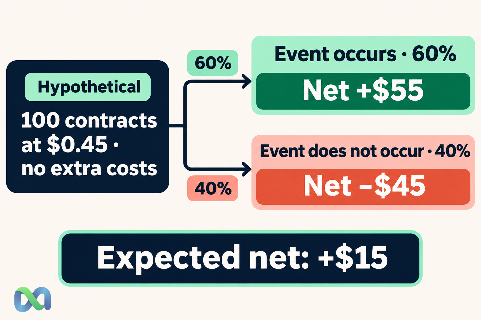
Assume a hypothetical purchase of 100 identical contracts at $0.45 each. Each pays $1 if one stated event occurs and $0 otherwise. Assume a 60% event probability, hold to settlement, and omit all extra costs solely for this teaching calculation.
The initial outlay is $45. If the event occurs, the total payout is $100 and net profit is $55. Otherwise, the payout is zero and net profit is −$45.
| Net | Chance | Weight |
|---|---|---|
| −$45 | 40% | −$18 |
| +$55 | 60% | +$33 |
| Expected result | — | +$15 |
Expected net profit is 0.40 × (−$45) + 0.60 × $55 = $15. The result is an average under the assumed probability, not a third possible settlement payoff. This position finishes at either −$45 or +$55 under the stated rules.
Its variance is 0.40 × (−45 − 15)^2 + 0.60 × (55 − 15)^2 = 2,400 dollars squared. Standard deviation is about $48.99. The variance guide explains why dispersion uses squared deviations rather than the average payoff alone.
All 100 contracts depend on the same event. Their settlement outcomes are not 100 independent Bernoulli trials. Confusing quantity with independent evidence would understate concentration risk.
Discrete Distribution Families to Know
Use a Bernoulli distribution for one binary indicator. Its parameter p is the chance of the outcome coded as 1. That coding does not automatically turn p into the chance of earning a positive net return.
A binomial distribution counts successes in a fixed number of independent trials with the same p. The fixed number of trials is central. A collection of contracts on correlated events is not binomial simply because every settlement is binary.
A geometric distribution describes the wait until the first success, using either trials or failures as the counting convention. Its assumptions include independent trials and a constant success probability.
A Poisson distribution models a count under a stated event-arrival structure. Its suitability requires more than observing whole numbers. Clustering, varying intensity, and dependence can make a simple Poisson assumption unsuitable.
These families are starting points for explicit questions. They are not interchangeable templates to apply to every column of a spreadsheet.
Continuous Distribution Families to Know
A uniform distribution gives equal probability to equal-width intervals within its support. It represents a substantive equal-density assumption. Knowing only a minimum and maximum does not prove that all interior intervals are equally likely.
An exponential distribution models a nonnegative waiting time with a constant hazard rate. That memoryless structure is restrictive. A changing arrival rate or a scheduled deadline may require another model.
A normal distribution is symmetric and extends indefinitely in both directions. It can be useful for some measurements or averages, while providing a poor description of bounded variables, strong asymmetry, or unusually heavy tails.
A lognormal distribution has positive support and can arise from multiplicative models. It can represent some positive quantities, but a net return that can be negative cannot itself follow an ordinary lognormal distribution.
The central limit theorem concerns suitable sums and averages under stated conditions. It does not mean that every underlying financial variable is normal or that a large spreadsheet removes dependence.
How to Choose a Distribution for a Financial Question
Start with the decision. Are you estimating a settlement probability, sizing a cash reserve, or describing execution delays? Specify what would count as a data point and which future situation the model is intended to represent.
Then identify structural restrictions. Counts cannot be negative. A probability lies between zero and one. A positive price and a signed price change have different support. Rules can also create point masses, such as a zero payment when an event does not occur.
Next, inspect how the data were collected. Repeated measurements of one event can be highly dependent. Data points from different policy regimes may not share the same distribution. A sample containing only completed or profitable positions can be biased before any fitting begins.
Finally, compare the model with held-out data points and alternative assumptions. Look at the feature that matters to the decision, especially tail probabilities or shortfall risk. A good fit near the center does not establish an accurate probability for rare losses. Document where the model performs poorly instead of hiding that uncertainty behind extra decimal places.
Use the Distribution Without Treating It as a Forecast Guarantee
Once the model is defined, calculate the quantity the decision actually needs. That might be an expected payoff, an interval probability, or a quantile. The expected value formula guide supplies the link between probabilities and payoffs.
Keep the event model separate from the trading implementation. Fees, spread, slippage, funding, liquidity, and settlement rules can change the payoff distribution even when the event probability is unchanged. A correctly calculated distribution for an idealized contract may still omit the main risk of an actual position.
Write down what would invalidate the model: a changing probability, a new dependency, a support violation, or an unmodeled loss mechanism. Revisit those conditions when new information arrives. Precision is useful only when the object being measured and the assumptions supporting it remain clear.
Frequently Asked Questions
What is the difference between probability and a probability distribution?
A probability describes one event. A distribution describes how probabilities are assigned across the possible values of a random variable. It can answer many event questions once the variable and model are stated.
Which distribution should a prediction market use?
There is no single universal answer. One binary settlement can be represented by a Bernoulli indicator. A portfolio, event count, or time to execution requires a different variable and possibly a different model.
Can two distributions have the same expected value?
Yes. They can share a mean while having different loss probabilities, dispersion, or tail exposure. Expected value is one summary, not a complete description of uncertainty.
Does more data guarantee the correct distribution?
No. More data points can improve estimation under suitable conditions, but they do not automatically correct biased sampling, dependence, changing regimes, or an unsuitable model family.
