


Probability Density Function: Meaning, Formula and Examples

A probability density function describes how probability is distributed across the possible values of a continuous random variable. The height of the function at a point is a density. The probability of an interval is the area under the curve across that interval.
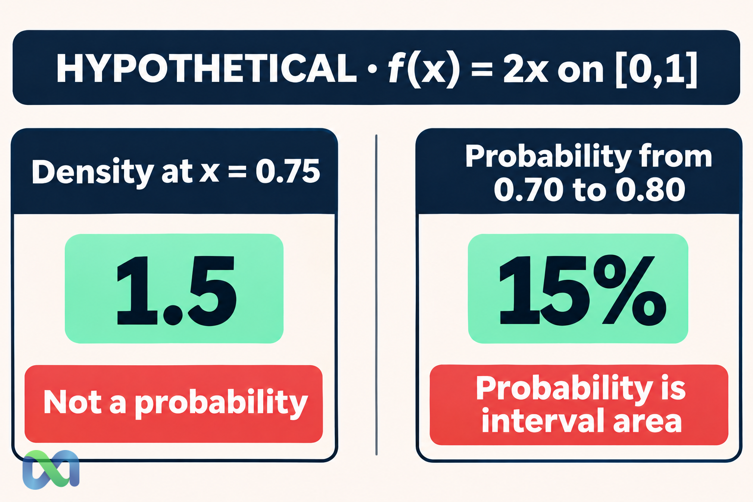
That distinction explains a common puzzle: a density can exceed one even though a probability cannot. In the illustrative model f(x) = 2x for 0 ≤ x ≤ 1, the density at x = 0.75 is 1.5, while the probability that X lies between 0.70 and 0.80 is only 0.15, or 15%.
This guide works through the density, cumulative distribution, mean, and interval probabilities of that model. It also explains when a probability mass function is needed instead, including for a binary contract’s final payout.
What Is a Probability Density Function?
For a continuous variable with a density f, the probability of falling between a and b is:
P(a ≤ X ≤ b) = ∫ from a to b f(x) dx
A valid density is nonnegative and has total integral one over its support. Values outside the support contribute no probability. The density’s height depends on the units used for x, whereas the probability of the corresponding event does not.
OpenStax’s continuous-probability lesson develops probability as area. For a continuous model, a single exact point has zero probability even if its density is positive.
The acronym PDF means probability density function in this context. It is unrelated to a document file format. In a statistical report, write out the term on first use and identify the random variable so readers know what the curve measures.
Not every distribution has a density of this kind. A discrete distribution uses point probabilities. A mixed distribution can have both continuous regions and probability concentrated at particular values. The type of variable determines which representation is appropriate.
A Valid Density: Check the Two Conditions
Consider the hypothetical density f(x) = 2x for x between zero and one, and f(x) = 0 elsewhere. This model puts more density near one than near zero. It is an illustrative distribution, not a fitted financial risk model.
First, the density is nonnegative throughout its support. Second, its total area is:
∫ from 0 to 1 2x dx = [x²] from 0 to 1 = 1
Both conditions hold. By contrast, using f(x) = x on the same support gives total area one-half, so it would not be a complete probability density without rescaling or specifying additional probability elsewhere.
You can imagine X as a modeled fraction of a fixed exposure lost in a hypothetical scenario. The model explicitly restricts that fraction to zero through one and emphasizes larger fractions. It is not suitable for a variable that can include gains, losses beyond the assumed exposure, or discrete default outcomes without further specification.
This interpretation illustrates why support is substantive. Drawing a smooth curve does not establish that it covers the possible outcomes of the actual quantity you want to study.
Worked Example: Calculate an Interval Probability
To find the probability that X lies between 0.20 and 0.60, integrate the density over that interval:
P(0.20 ≤ X ≤ 0.60) = [x²] from 0.20 to 0.60
= 0.60² − 0.20² = 0.36 − 0.04 = 0.32
Thus the probability is 32% under the hypothetical model. If X represents the illustrative loss fraction, this event corresponds to losses between 20% and 60% of the fixed exposure. It is not a statement about observed losses or an actual position.
Other intervals can be calculated in the same way:
| Interval | Probability |
|---|---|
| 0–0.20 | 4% |
| 0.20–0.60 | 32% |
| 0.60–1 | 64% |
These regions cover the full support, and the probabilities sum to 100%. The shared endpoints cause no double-counting in this continuous model because point probabilities are zero.
The region above 0.60 has more probability than the equally wide region from zero to 0.40. The density rises with x, so equal widths need not have equal areas. A flat density would be a different distribution.
Density Height Is Not Point Probability
At x = 0.75, the model gives f(0.75) = 1.5. This does not mean a 150% probability. The density measures probability per unit of the x scale, and it must be integrated over an interval to produce a probability.
For the interval from 0.70 to 0.80:
P(0.70 ≤ X ≤ 0.80) = 0.80² − 0.70² = 0.15
Here, multiplying the midpoint density 1.5 by the width 0.10 also gives 0.15 because the density is linear. For a nonlinear density, midpoint height times width is generally an approximation, not an exact universal rule.
At one exact value, P(X = 0.75) = 0 in the continuous model. Observing a rounded value such as 0.75 is a different event if the measurement device reports a range as that rounded number. The recorded category can have positive probability even though an exact mathematical point does not.
Changing the measurement units changes density height. Expressing a fraction as a percentage rescales the horizontal axis and changes the density per horizontal unit. Areas for matching real-world intervals remain the same.
PDF vs. CDF
The cumulative distribution function is F(x) = P(X ≤ x). It accumulates probability from the lower end of the support to x. A CDF is nondecreasing and takes values between zero and one.
For the worked model, F(x) is zero below zero, equals x² for 0 ≤ x ≤ 1, and equals one above one. Thus F(0.60) = 0.36. Subtracting F(0.20) = 0.04 recovers the 32% interval probability.
Where the required derivative exists for this continuous model, the density is the derivative of the CDF. Differentiating x² produces 2x. Integrating the density reverses that relationship.
NIST’s probability-distribution overview distinguishes continuous density and discrete probability descriptions. Keep the representation and units clear when comparing plots. A rising CDF does not mean the density is rising: every valid continuous CDF accumulates area, even where its density is falling.
Mean, Variance, and Quantiles from a Density
An expected value weights each possible value by its density. For the example:
E[X] = ∫ from 0 to 1 x × 2x dx = 2/3 ≈ 0.6667
The second moment is E[X²] = ∫ from 0 to 1 x² × 2x dx = 1/2. Therefore the variance is 1/2 − (2/3)² = 1/18 ≈ 0.05556, and the standard deviation is approximately 0.2357.
The variance guide explains why the second moment alone is not the variance: the squared mean must be subtracted. The mean is also not necessarily a point of highest density. In this example, density increases toward the upper boundary while the expected value remains two-thirds.
To find the q quantile, solve F(x) = q. Here x² = q, so xq = √q. The median is approximately 0.7071, and the 90th percentile is approximately 0.9487. These describe the hypothetical distribution itself, not confidence intervals estimated from a sample.
PDF vs. Probability Mass Function
A probability mass function, or PMF, assigns probabilities to discrete values. If a binary contract pays one unit when an event occurs and zero otherwise, its final gross payout has probability mass at zero and one under a specified event probability. A smooth density over every intermediate payout would describe a different variable.
Likewise, the binomial distribution assigns probability to integer success counts. Its plotted bars are point masses, not pieces of a continuous density. Adding the relevant masses gives an event probability.
A continuous variable can use interval areas, while a discrete variable uses sums. A mixed model might include a positive probability of no loss together with a continuous range of positive losses. Ignoring the point mass would omit part of the distribution.
Separate a contract’s final payoff from its changing market quote, a modeled loss fraction, or a forecast estimate. Those quantities can have different supports and different distributions even when they concern the same underlying event.
Reading a Density Plot in Financial Research
Check the horizontal variable, units, support, and source of the curve before interpreting its height. A theoretical density is a model. A histogram summarizes observed bins. A smoothed density estimate depends on choices such as bandwidth and boundary treatment.
A peak at one value does not by itself identify the most probable interval unless the intervals being compared have equal width. An upper-tail risk question requires the integrated tail area, rather than the height at a single threshold.
A model can also smooth away economically important point masses or assign probability to impossible values. For example, a normal approximation can extend beyond a hard boundary. Assess whether that mismatch matters for the calculation you intend to make.
Our normal distribution guide provides a familiar continuous example. The Monte Carlo simulation guide explains how repeated draws can estimate probabilities within a model without proving that its density matches real outcomes.
Calculate the Example in a Spreadsheet
For a threshold x in cell B2 within zero through one, =B2^2 gives the CDF and =2*B2 gives the density. In an English-language spreadsheet, a CDF formula covering all thresholds is =IF(B2<0,0,IF(B2>1,1,B2^2)).
For the interval 0.20 to 0.60, use =0.6^2-0.2^2. For a simulated draw from this particular distribution, transform a uniform random number using =SQRT(RAND()). Applying the inverse CDF produces the intended rising density rather than a uniform output.
Confirm that interval limits are in the correct order and within the model support, or clip them appropriately before integrating. Keep density and cumulative-probability columns clearly labeled. A correct density value entered where a probability is expected can still produce an invalid downstream risk calculation.
Frequently Asked Questions
Can a density be negative?
A valid probability density is nonnegative. A proposed function that becomes negative over a region of positive width cannot represent a probability density there without changing the specification.
Why does a point have zero probability?
An exact point has no width, so its area under a continuous density is zero. A measurement rounded to a particular number can represent an interval, which can have positive probability.
Does every distribution have a PDF?
Not in the ordinary continuous-density sense. Discrete distributions use mass functions, and mixed distributions need both continuous and point-mass components. Identify the variable and its possible outcomes before choosing the representation.
